Introduction
The Japanese PM dissolved the lower parliament on 28th September, initiating the process for the snap elections to be held on October 22nd. We believe that it is a move to secure a fresh mandate in the parliament after Mr. Abe’s association with a series of scandals over the summer. The approval rating for Abe’s government sunk to 29.9%, sliding below 30% for the first time, and his disapproval rating rose to 48.6% [according to a poll conducted by the Jiji news agency]. Japan has been stuck in an on-and-off cycle of deflation for two decades now and the election is an opportunity for the people to re-affirm their belief in the sustenance massive economic stimulus that drives the nation.
While Mr. Abe’s party is likely to come out of the elections unharmed, the results might deviate for the worse due to Yuriko Koike, the popular governor of Tokyo. The 65-year-old Ms Koike was an environment minister and defence minister in the LDP before she defied Mr Abe last summer, ran against his candidate for the Tokyo governorship and won in a landslide. She set up a local party called Tomin First and in July it won a sweeping victory in elections to the Tokyo assembly. She has created a new “Party of Hope” to challenge the duopoly that has dominated Japanese politics. The new group, includes some defectors from both Abe’s Liberal Democratic Party and the opposition Democratic Party. According to one recent poll carried out by Nikkei Newspaper Mr Abe’s LDP is supported by 44 per cent of voters, with the opposition Democratic party on 8 per cent and the Party of Hope also on 8 per cent. While the percentages put Mr. Abe’s LDP well ahead of the others, analysts fear that key seats could be lost due to Yuriko Koike’s well-established fan-base.
Mr Abe’s policy platform of raising taxes to spend on the young suggests that his campaign will be fought along populist lines. It is well aimed at exploiting a weak opposition, rather than winning a mandate for painful economic reforms or drastic constitutional change. He has also ordered his cabinet to prepare a ¥2tn ($17.8bn) fiscal stimulus package before the end of the year. A pillar policy of his manifesto will be a pledge to raise consumption tax from 8 per cent to 10 per cent in 2019, and redirect much of the money to provide free childcare for 3-5 year olds. Ms. Koike, on the other hand, needs to carve a political space for herself for most of her policies are much in line with that of Mr. Abe.
The opposition, in general, is struggling to coalesce around centrist candidates with nationwide appeal. Ms. Koike backs constitutional reform, increasing the odds that supporters of a change will secure the two-thirds parliamentary majority needed to pass a revision, and then take it to a national referendum for approval. Ms. Koike has not given a clear indication whether she would pursue economic reforms like those promised by Mr. Abe in 2012. Given her political career and history, she is mainly interested in reforming government rather than liberating the private economy from heavy regulation and taxes.
Given the turbulent and scattered nature of the opposition’s agenda, pollsters suggest Mr. Abe should come out unscathed with a probable loss of few seats. His party has a formidable electoral machine, the economy is doing well and Japan’s public appreciates the five years of political stability the prime minister has brought. Economic growth in the second quarter was also surprisingly strong by Japanese standards, with real GDP rising 2% year on year.
The markets are expected to respond well to Shinzo Abe’s re-election. His five principle policies of acceleration of Abenomics, a VAT hike with the reallocation of tax revenue to education, enhancement of the work-style reform, constitutional reforms Japan’s constitution (including the revision of Article 9), and measures against the North Korea crisis are all positive sentiments. In the next section, we will explore some market trends that have been seen in previous snap elections.
Event Strategy
The event of a snap election is not uncommon for the Japanese politics: in the post-word period, only one election, in 1976, has been triggered by the natural expiration of the parliamentary term. Looking at historical data, at a first glance, it seems that the stock market usually reacts positively to the announcement of a snap election, pointing to a stronger government. Usually, however, just after the election the market corrects its over-confidence on the possibility of a strong mandate, and returns lower in the period following the election [1].
In order to verify this idea, we performed an event study with the data of both Nikkei 225 and TOPIX indexes. These indexes have different characteristics – both in terms of components and in terms of weighting. In particular, the Nikkei 225 is a price-weighted index, while the Topix is a free-float weighted index: in this sense, they can be compared to the Dow Jones and S&P 500 respectively.
An event study is a process used to determine the effects of a certain event on the returns of an asset. A common applications of event studies is the analysis of the effect of M&As on the stock price of either the acquiring or acquired company. In order to effectively perform an event study, one needs to clearly determine a number of objects. First, the event window – a set of days around the event – and the estimation window – a different set of days that ends before the event window. Usually a post-event window is also used. The event window coincides with the period over which we expect to see the effect of the event on the returns of the asset of interest. The estimation window, instead, is used to estimate the expected returns over the event window. As a matter of fact, we are not interested in the returns per se around the event, but just on the “abnormal returns”, that is on the actual returns minus the expected returns, conditional on the event never happening. Different ways have been suggested to estimate expected returns: in this case we shall use the simple constant return model, which has proven to perform at a level comparable with that of more complex models. Finally, the results need to be tested through a statistical test, to see whether abnormal returns are consistent with the model for expected returns or not. We shall perform two different kinds of tests.
In our analysis, we considered all 18 snap elections that happened since 1960. As we couldn’t obtain the exact dates in which all elections were called, we consider event windows of 35 trading days for all elections, which means c. 49 calendar days. This is slightly more than the election periods of which we have data – that show an average of 30 and a maximum of 40 calendar days since the dissolvement of the House until the election day. By using a larger window, we hope to avoid the exclusion from the event window of the day in which the election was called, which is expected to show a return greater than usual (in absolute terms). Also, since there are usually rumours of the election been called some days before the announcement, we consider this to be a more consistent approach.
We have defined our event window. In order to estimate the expected returns over this period, we use a window of the same length, ending the day before the event window starts. The average of the log returns over the estimation window gives the expected daily return for the event window it refers to. By assuming independency of returns, the expected cumulative return over the entire event window coincides with the daily expected return times the length of the event window. Daily abnormal returns are given by the difference between the actual return of the day and the expected daily return. We have obtained, therefore, a set of 18 times series of abnormal returns for each index, which last 35 trading days each. The table below shows the cumulative abnormal (log) returns (CAR) for each election.
| Election | Nikkei 225 CAB | TOPIX CAB | Election | Nikkei 225 CAB | TOPIX CAB |
| 20/11/1960 | -3,62% | -5,51% | 18/02/1990 | -6,60% | -5,78% |
| 21/11/1963 | 0,42% | 0,19% | 18/07/1993 | -6,45% | -8,16% |
| 29/01/1967 | 2,83% | 4,78% | 20/10/1996 | 8,27% | 6,27% |
| 27/12/1969 | 2,83% | 4,25% | 25/06/2000 | 10,42% | -1,13% |
| 10/12/1972 | 3,16% | 7,93% | 09/11/2003 | -11,10% | -12,41% |
| 07/10/1979 | -3,43% | -2,81% | 11/09/2005 | 6,01% | 7,17% |
| 16/05/1980 | 4,35% | 5,67% | 30/08/2009 | 10,81% | 10,10% |
| 18/12/1983 | 1,95% | 3,26% | 16/12/2012 | 12,57% | 11,21% |
| 06/07/1986 | 2,75% | 2,77% | 14/12/2014 | 9,38% | 9,57% |
Table 1 (Source: BSIC, Bloomberg)
In addition to this, we consider a “post-event window” of 25 days starting after the election. According to our theory, we expect returns to be lower than those experienced in the previous period. We compute the same procedure as before: we estimate the expected return, and subtract it from the actual one for each day of the post-event period. Since we want to test whether returns in this period are smaller than those in the previous one, we use as expected daily return for the post-event window the average daily return occurred in the event window. In the table below, we show cumulative (log) abnormal returns (CAR) for each post-event window.
| Election | Nikkei 225 CAB | TOPIX CAB | Election | Nikkei 225 CAB | TOPIX CAB |
| 20/11/1960 | -4,47% | -8,17% | 18/02/1990 | -20,04% | -19,82% |
| 21/11/1963 | -5,10% | -2,53% | 18/07/1993 | 4,37% | 1,60% |
| 29/01/1967 | 3,23% | 0,31% | 20/10/1996 | -6,26% | -5,26% |
| 27/12/1969 | -7,69% | -7,02% | 25/06/2000 | 0,41% | -0,05% |
| 10/12/1972 | -0,32% | 0,48% | 09/11/2003 | -2,58% | -2,73% |
| 07/10/1979 | -3,48% | -4,30% | 11/09/2005 | 1,21% | 3,46% |
| 16/05/1980 | -2,11% | -2,58% | 30/08/2009 | -13,84% | -14,84% |
| 18/12/1983 | 4,92% | 6,14% | 16/12/2012 | 2,36% | 5,27% |
| 06/07/1986 | -9,51% | -1,70% | 14/12/2014 | -9,97% | -9,99% |
Table 2 (Source: BSIC, Bloomberg)
In the chart below, finally, we plotted the path of two theoretical investments that bought the index (TOPIX and Nikkei 225 respectively) 70 days prior to each election. The “0” value on the X axis corresponds to the election date, while the “-35” corresponds to the theoretical date in which the election was called: the start of the event window. At a first glance, results seem to confirm our theory. After the election is called, there is a significant increase in the mean returns, that ends right before the election day: in the subsequent period, returns are on average slightly negative.
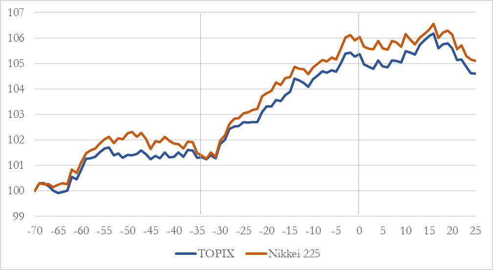
Chart 1 (Source: BSIC, Bloomberg)
Therefore, we proceed with a more formal statistical testing. We first conduct a simple t-test on the “average” cumulative distribution. Then, we first present and then apply a more precise test, that takes into account the sampling variance of the expected return. The t-tests is performed on the following hypothesis:

In words, we test whether the mean of the cumulative abnormal returns of the event windows is equal to 0, or if it is instead positive. Then, we perform the same test on the post-event window, under the hypothesis:

The results are as follow:
| Event window | Nikkei 225 | TOPIX |
| T-stat | 1.81 | 1.70 |
| P-value | 4.41% | 5.36% |
Table 3 (Source: BSIC)
| Post-event window | Nikkei 225 | TOPIX |
| T-stat | -2.94 | -2.91 |
| P-value | 0.62% | 0.65% |
Table 4 (Source: BSIC)
Based on this test, we reject both null-hypothesis and conclude that returns significantly increase between the announcement and the election day, and decrease right after it.
We now propose a second, more rigorous test, in the sense that includes into the variance of the cumulative abnormal return, the variance of the estimator of the expected return. This comes from the fact that the expected daily return is not known “a priori”, but is estimated as the mean of the returns in the estimation window. The variance of this estimate has to be “summed” to that of the actual return. More formally, call:

the vector of abnormal returns for the election i, where is the vector of actual returns, a vector of 1 and the estimate of the mean daily returns. Under the null hypothesis, the abnormal returns will be jointly normally distributed, with expected value of 0 and covariance matrix:

Where I is the identity matrix with dimension equal to the number of observations in the event window, is the variance of dailies returns and a vector of 1 with dimension equal to the number of days in the estimation window. Now we can define the cumulative abnormal return as the sum of the dailies abnormal returns, or:

Under the null, this is distributed as a normal distribution with expected value 0 and variance:

We can see that the variance decreases with the length of the estimation window (because of ): with the increase of the estimation window, the estimate of the expected returns becomes increasingly precise. Finally, the mean cumulative abnormal return ( is normally distributed with expected value 0 and variance

The statistic:

is asymptotically distributed according to standard normal, and can be used to perform a classic Z-test. The results of the test applied to both the event and post-event window are shown in the table below.
| Event window | Nikkei 225 | TOPIX |
| J-stat | 1.28 | 1.20 |
| P-value | 10.04% | 11.45% |
Table 5 (Source: BSIC)
| Post-event window | Nikkei 225 | TOPIX |
| J-stat | -2.25 | -2.22 |
| P-value | 1.23% | 1.31% |
Table 6 (Source: BSIC)
As expected, these test shows an inferior level of significance compared to that of the simple t-test, especially for the event window. However, we believe that these results confirm our idea: before the election stock returns on average outperform the previous period, and after the election they decline compared to the growth shown in the prior period.
As a result, even though the election has been announced some days before, we suggest to be long on the Japanese indexes (as history shows that abnormal returns are positive for the entire period before the election day), and to sell them on the last trading day before the election.
[1] “Japanese stocks ready for Snap! Crackle! Pop!”, Financial Times (https://www.ft.com/content/9e5c32c6-a1e0-11e7-9e4f-7f5e6a7c98a2)


0 Comments