Introduction
Over the past decade, volatility as asset class has attracted the attention of several institutional investors, who consider it as an interesting hedge against long position in equities, given the evident negative correlation that persist between the two asset classes due to the leverage effect. Unfortunately, volatility indexes are not tradable, so investors gain exposure to this asset class through derivatives, such as futures, which are the protagonists of our analysis.
Clearly, the most important volatility index is the VIX, which was introduced in 1993, and it measure the market’s expectation of 30-day implied volatility derived from S&P 500 Index options. The VIX has been widely used as a fear market sentiment, with high values indicating market stress and low values indicating calm market conditions. Ever since, a new set of volatility indices have been developed to capture market sentiment in other major markets. Among them we are considering the VSTOXX for the Eurozone, the VXEEM for emerging markets, and the VHSI for Hong Kong equities.
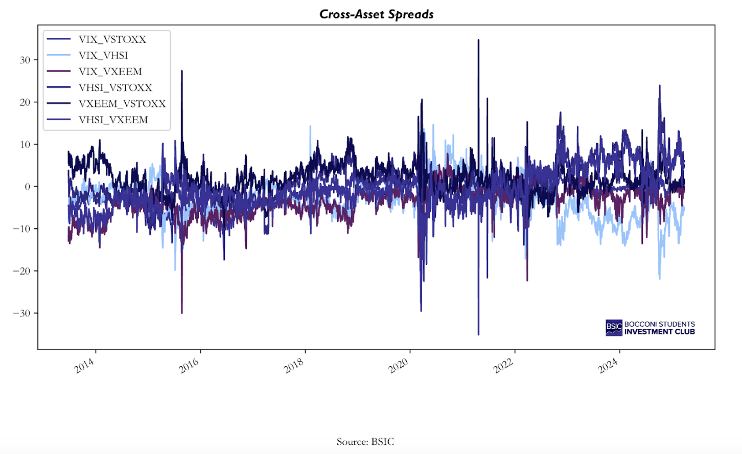
These indexes reflect their local market conditions; however, their movements are often interconnected, as demonstrated by their correlation coefficients, which range from 65% for the VSTOXX-VHSI pair to 86% for the VIX-VSTOXX pair. In this article, we extend previous analysis on volatility futures by Stanescu and Tunaru (2013), by examining the statistical properties of the spreads between the 4 volatility indexes, with the spreads being defined as a simple difference between the prices of indexes’ futures. Using statistical tests and GARCH modeling, we assess whether these spreads exhibit mean-reversion and whether volatility clustering can be exploited to predict the evolution of the spreads. The main idea is to apply autoregressive and conditional variance models to capture the mean and the volatility dynamics of the spreads, following the methodology of Stanescu and Tunaru (2013). The goal is to evaluate whether the statistical features of these spreads can justify a systematic trading strategy.
Modelling Volatility Indices Spread
We begin by reporting the main statistical properties of the spreads, along with the results from the t-test for the mean, the ADF and PP tests for stationarity; and the ARCH-LM for conditional heteroskedasticity.
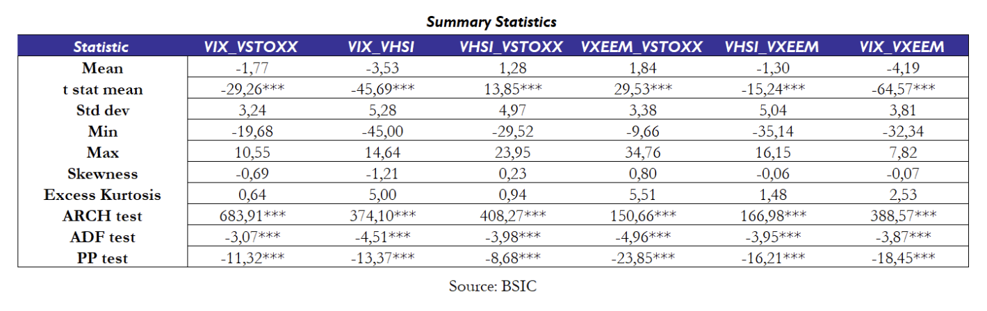
Preliminary results show that all the spreads are significantly different from zero, as highlighted by the t-stat statistic. On top of that, we can reject the null hypothesis of a unit root in the timeseries, given that both the ADF and PP test are significant at any confidence level. This means that the spreads are stationary and exhibit mean-reverting behaviour over time. Notably, the excess kurtosis is positive for every spread, meaning the distributions present fatter tails compared to a normal distribution, which will make us opt for a GARCH model with student-t innovations in the following section. Finally, also the ARCH tests statistics are highly significant, indicating the presence of conditional heteroskedasticity and justifying the application of GARCH models.
Given all the above, we decided to test several models to capture the tendencies in the data. For the conditional mean of the spreads, we specified an autoregressive model of order 4 AR(4), supported by autocorrelation and partial autocorrelation analyses (ACF and PACF), which show significant lags up to four periods. Formally, the AR(4) model for the spread yt is defined as:

Where εt represent the residuals, so the unexpected shocks not captured by the autoregressive model. These residuals are what we used to estimate conditional volatility trough the GARCH model. In particular, we tested a GARCH(1, 1) specification, both with Normal and Student-t innovations. The standard GARCH(1, 1) process is given by:

So, the conditional variance is modelled as a linear combination of t-1 squared shocks and squared variance itself. The idea of this kind of model is to capture a very well-known phenomenon in empirical finance, which is volatility clustering, meaning that periods of high volatility are followed by high volatility, and the same for low volatility periods.
Actually, we also tested the so called GARCH-in-mean model, which includes the forecast of the conditional volatility in the mean equation, hoping that higher of lower uncertainty has a measurable effect on the level of the spread itself. Formally, the model is just an extension of the AR model, since it adds the term  :
:

A positive and significant γ would imply that higher volatility tends to widen the spread, suggesting the presence of volatility risk premium. What we observe is consistent with Stanescu and Tunaru [1], who didn’t find statistical significance in this coefficient for the VIX-VSTOXX spread. However, we actually found that the coefficient of the conditional volatility is significant for the VIX-VXEEM, VXEEM-VSTOXX, and VHSI-VXEEM spreads and borderline significant for VHSI-VSTOXX (p-value 5.07%). Overall, this suggests that adding the conditional volatility to the mean equation could be beneficial when the VXEEM index is involved. In any case, we decided to stick to the AR(4) + GARCH(1, 1) with Student-t innovation to model each pair for consistency with Stanescu and Tunaru methodology and for consistency among the pairs. The in-sample results are provided in the following table:
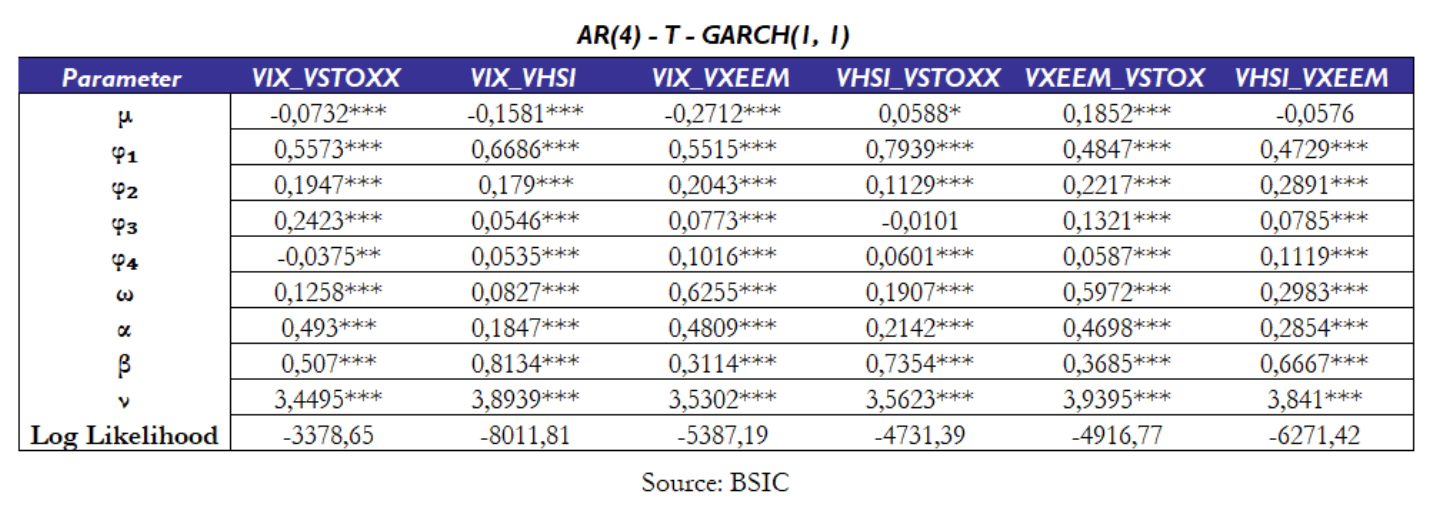
With only few exceptions, all the coefficients of the regressions are statistically significant, confirming our modelling approach is a good fit for the data. Notably ν, which represent the degrees of freedom of the Student-t distributions ranges between 3.4495 and 3.9395 and it’s statistically significant at any confidence level, supporting the choice of modelling the spreads with Student-t, rather than Normal innovations. Overall, the in-sample estimation results demonstrate that the AR(4)–GARCH(1,1) model under Student-t innovations provides a robust and statistically sound framework to describe the dynamics of volatility spreads across regions.
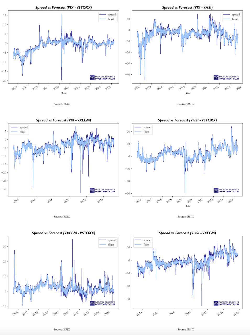
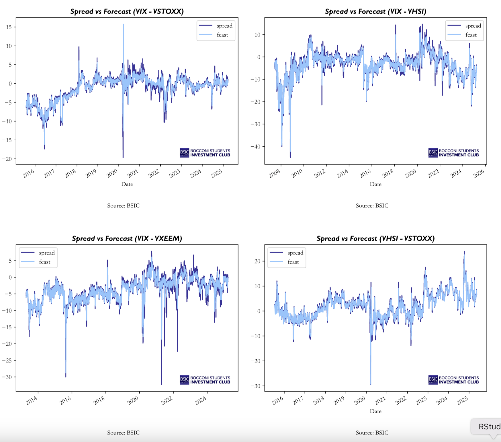
To develop a systematic trading strategy, we need a model which is capable of delivering consistent out-of-sample results. Therefore, we employed a rolling-window forecasting framework, where at each point in time (t), we re-estimate the AR(4)-GARCH(1, 1) model using a 500-day moving window. The estimated models are then used to compute the t+1 forecasts of both the conditional mean and conditional variance. This procedure ensures no look-ahead biased is introduced and allows the model parameters to adapt over time to evolving market conditions. So, the t+1 change in spreads is computed by subtracting the spreads at time t from the forecasted spreads at t+1. This measure is then standardized by the forecast of conditional volatility, which finally results in our trading signal. The standardized forecasted change represents the expected movement of the spread in units of its own conditional volatility, so it provides a risk-adjusted measure of how large the predicted deviation from the current level of the spread is going to be. A positive signal implies the spread is expected to increase, suggesting a long position in the first leg and a short position in the second leg (for example, long VIX and short VSTOXX). Conversely, a negative signal indicates an expected decrease in the spread, which indicates the opposite position. Then, the absolute value of magnitude of the signals indicates the “confidence” in the predictions: higher values indicate the forecasted change is large compared to its expected risk, while lower values indicate that the forecasted change is small relative to the expected volatility, hence statistically less meaningful. The plots and main metrics of the out-of-sample forecasting are presented below.

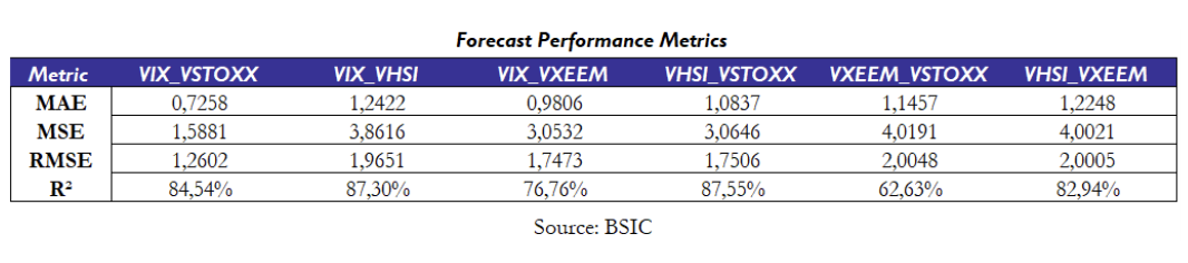
Overall, the AR(4)-GARCH(1, 1) model delivers strong out-of-sample forecasting performance, across all volatility spreads. As shown in the figures, the predictions closely track the actual spreads. From a quantitative point of view, forecast errors, captured by Mean Average Error (MAE), Mean Squared Error (MSE), and Root Mean Squared Error (RMSE) remain low and the explanatory power (R2) of the model is high. In particular, the table show very promising out-of-sample results for VIX_VSTOXX, VIX_VHSI, VHSI_VSTOXX and VHSI_VXEEM, while the worst performing spread is the VXEEM_VSTOXX pair, which show a low R2 (62.63%) compared to the other pairs.
Strategy Overview
We implement the strategy trading cross-country spread over different volatility indices. We use prediction from the model previously described. Model parameters are re-estimated daily, using a rolling sample of 500 observations. Given one day ahead forecast we enter a narrowing trade when the model predicts a decrease in the spread, and a widening trade when it predicted an increase.
For each leg of the trade, we go either long or short futures contracts of the volatility indices with a size equivalent to 100.000$. Fixed transaction costs of 3 bps were assumed, and the number of contracts were adjusted daily for currency exchange rate so that short and long position stayed the same.
Results
The out-of-sample backtest confirms that the model provides consistent, risk-adjusted performance across our vol index pairs. Starting with emerging market exposures, the VXEEM–VSTOXX pair (Fig. 1–2) delivered highly unstable performance with deep drawdowns and a negative cumulative PnL.
As illustrated in Fig. 1, profits show long negative periods ending in abrupt upswings, suggesting a fragile relationship between European and emerging market volatility. The Sharpe ratio (Fig. 2) remains well below zero for most of the period, reflecting the limited predictability of the spread. The underperformance here can also be attributed to a data limitation, that is, the lack of continuous VXEEM futures data. Consequently, this spread’s out-of-sample profitability should be interpreted with caution, as real returns would likely be lower.
Moving to the VHSI–VXEEM pair (Fig. 3–4), the results improve but remain volatile. Fig. 3 shows alternating cycles of sharp gains and losses, while the Sharpe evolution in Fig. 4 indicates only brief periods of statistical significance. These fluctuations could emphasize how volatility linkages between Hong Kong and emerging markets are weaker and less persistent than those between more representative macro indeces.
The VHSI–VSTOXX pair (Fig. 5–6) demonstrates greater stability and a persistent upward PnL trajectory. The Sharpe ratio in Fig. 6 consistently remains above one during multiple periods, suggesting that Asian and European implied-volatility spreads are more predictable and mean-reverting. This reinforces the conclusion that spreads between developed or financially integrated markets exhibit more robust dynamics.
The VIX–VXEEM pair (Fig. 7–8) stands out as one of the top performers in absolute terms, achieving a peak Sharpe of approximately 1.15. However, because this result is also based on VXEEM spot data, it likely overstates tradable profitability. In practice, if replicated with real futures, we would expect the naive strategy performance to converge to the same range as the VIX–VSTOXX spread (Sharpe ≈ 0.5–0.7), reflecting more realistic costs and volatility-term-structure effects.
The VIX–VHSI strategy (Fig. 9–10) produced moderate but consistent results. Its Sharpe ratios stay around 0.8, with limited drawdowns and a balanced exposure chart. The smoother performance shown in Fig. 9 highlights the strong co-movement between U.S. and Hong Kong volatility, consistent with global risk-off contagion effects.
The VIX–VSTOXX spread (Fig. 11–12) serves as a benchmark, replicating findings from Stanescu and Tunaru (2013). As shown in Fig. 11, cumulative PnL is positive and persistent, while Fig. 12 reveals a stable Sharpe ratio near 0.55, matching expectations for a well-behaved, low-beta volatility-spread trade.
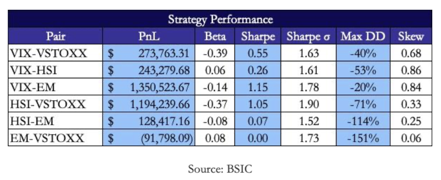
Despite the limitations, several robust features emerge:
- Low average betas (often negative) indicate that the spreads are largely uncorrelated with global equity risk and could serve as effective diversifiers in a multi-asset or traditional long-equity portfolio. This is something we look forward to exploring further
- Positive skewness across most pairs suggests the strategy tends to generate larger upside outliers than downside ones–consistent with mean-reversion structures where dislocations suddenly correct.
- Sharpe stability across pairs (Sharpe std. dev. ≈ 1.6-1.9) demonstrates resilience of the standardized signal construction, even when applied to heterogeneous regional markets.
In summary, while the results support the presence of profitable mean-reversion dynamics across volatility index spreads, they should be interpreted within the constraints of available data. Nonetheless, our findings suggest that cross-market volatility spreads remain a promising area to continue looking for opportunities in the realm of systematic strategy, especially between highly integrated developed markets.
Appendix
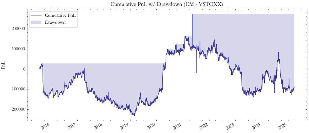
Fig. 1: Profit EM/VSTOXX
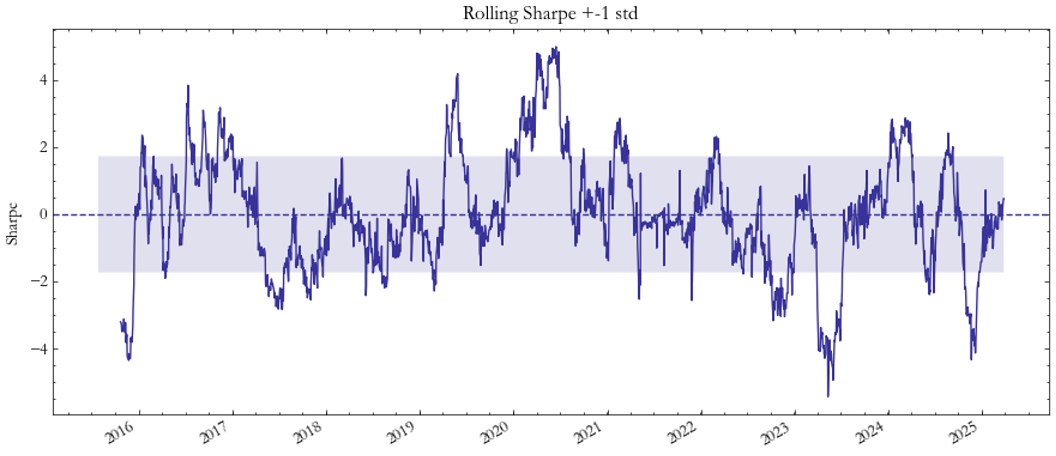
Fig. 2: Sharpe EM/VSTOXX
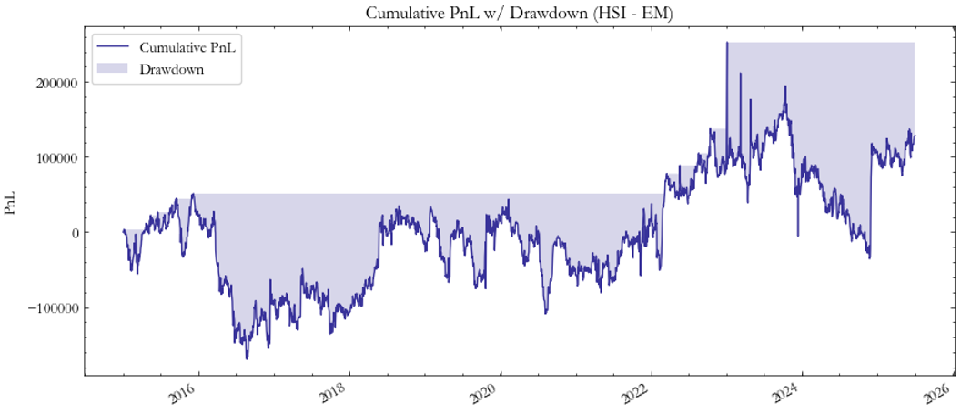
Fig. 3: PnL HSI/EM
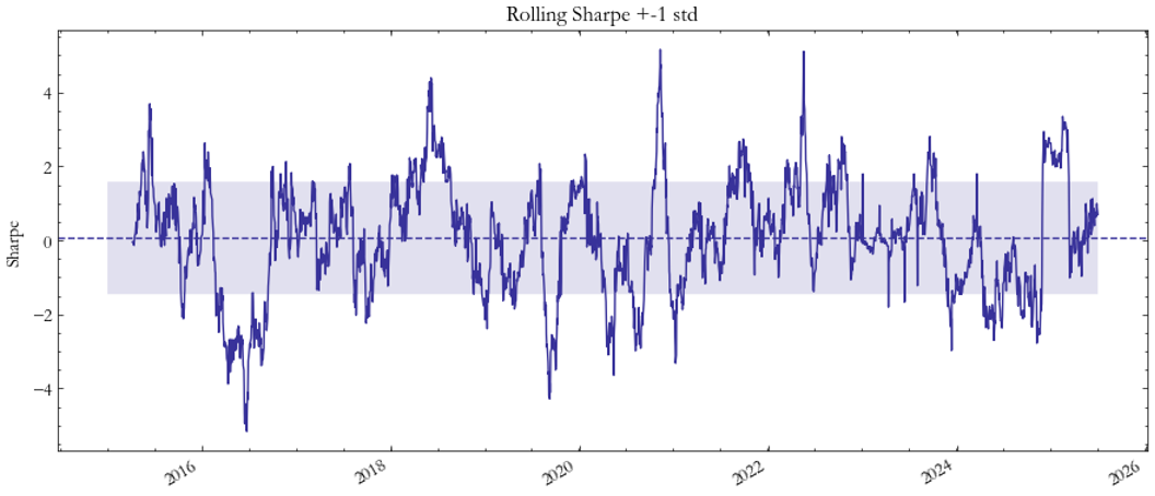
Fig. 4: Sharpe HSI/EM
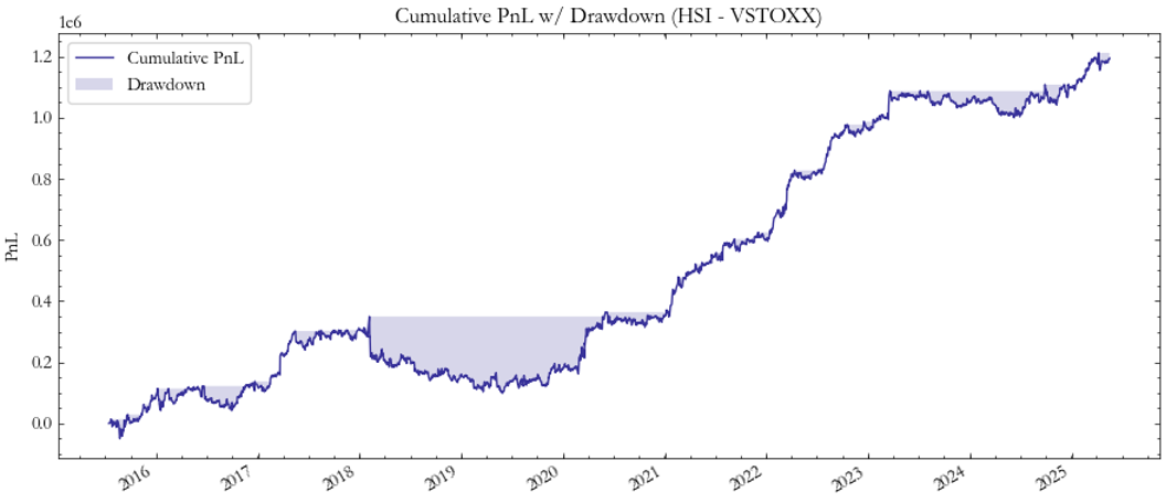
Fig. 5: PnL HSI/VSTOXX
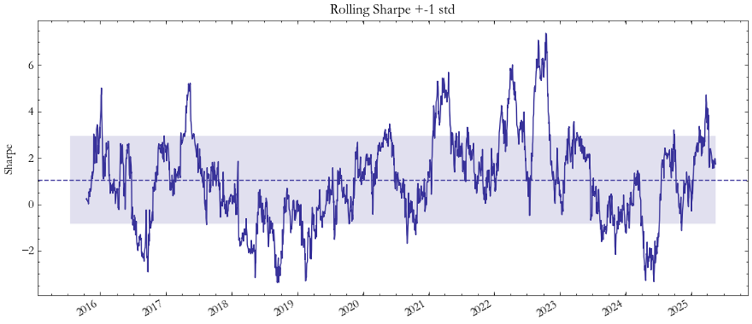
Fig. 6: Sharpe HSI/VSTOXX
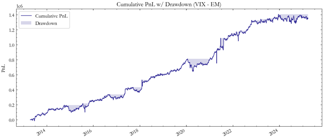
Fig. 7: PnL VIX/EM
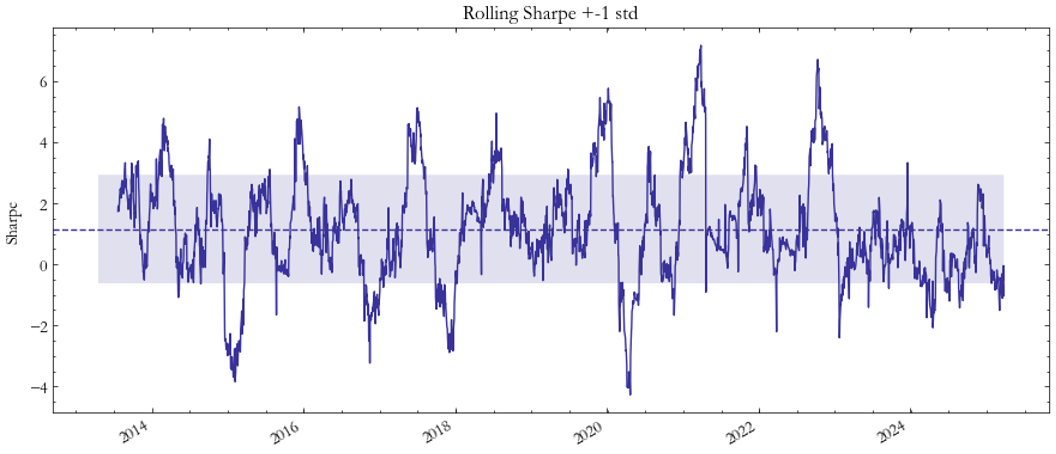
Fig. 8: Sharpe VIX/EM
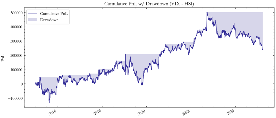
Fig. 9: PnL VIX/HSI
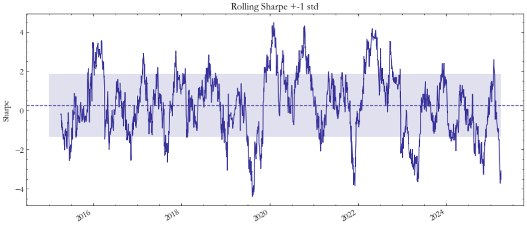
Fig. 10: Sharpe VIX/HSI
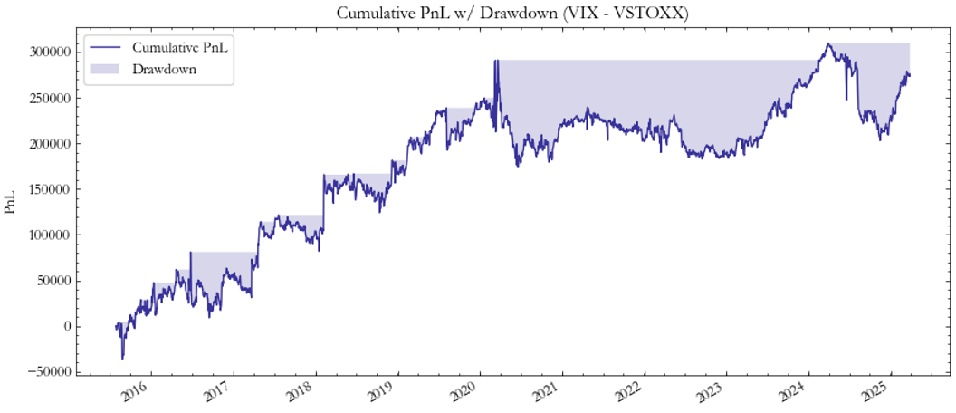
Fig. 11: PnL VIX/VSTOXX
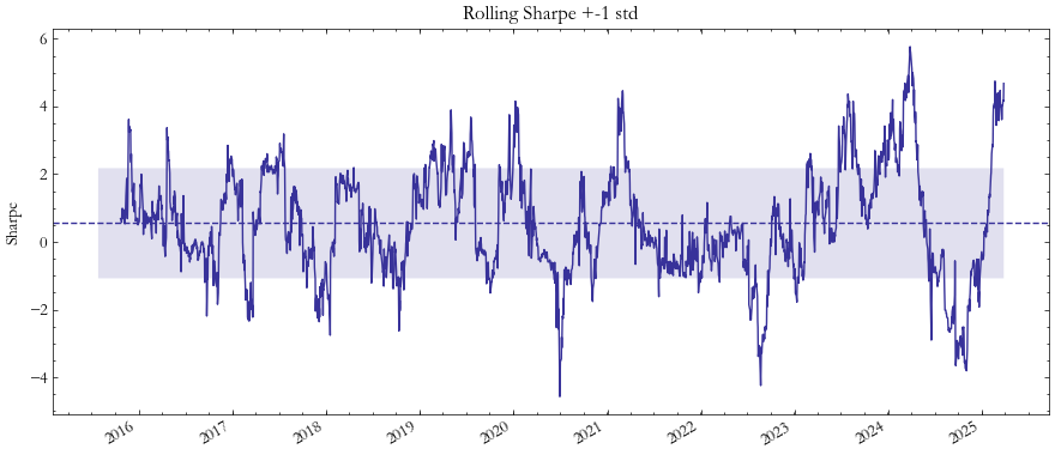
Fig. 12: Sharpe VIX/VSTOXX
References
[1] Stanescu, Tunaru, “Investment Strategies with VIX and VSTOXX Futures”, 2013


0 Comments