WHAT DRIVES CREDIT? Understanding the Cross Section of Expected Corporate Bond Returns

Abstract

While the literature investigating risk premia driving the cross section of stock returns is extensive, fewer studies analyze corporate bond returns. We set out to understand which factors and firm characteristics command a premium in terms of expected returns on corporate bonds, both in the investment grade and high yield spaces. We include a broad array of risk exposures ranging from financial characteristics to the macroeconomic environment. This is the first part of a two-part paper, where we will also perform statistical estimation. We start with a discussion of the theoretical foundations that make this stream of research in empirical asset pricing possible, then we propose a framework to analyze the cross section of expected corporate bond returns. We introduce two new factor proxies which, to our knowledge, have not been proposed in previous studies.

Introduction

The Arbitrage Pricing Theory (APT) developed by Ross [1] (see Huberman [2], Campbell [3] or Cochrane [4] for a deeper discussion) starts with an assumption on the distribution of asset returns in competitive and frictionless markets. Given a risk-free (or zero-beta) return $r_0$ , the distribution is described by the linear factor model (We use the unconditional formulation where the factor loadings are time independent).

$r_{i,t} - r_{t}^f = \alpha_i + \sum_{k=1}^K \beta_{ik} f_{kt} + \varepsilon_{it}$

where

$E(\varepsilon_i \varepsilon_j) = E(\varepsilon_i) = 0, \quad i \neq j, \quad i,j = 1, \ldots, N$

$E(\varepsilon_i^2) < \infty, \quad i = 1, \ldots, N$

$E(F_k \varepsilon_i) = 0, \quad k = 1, \ldots, K, \; \; i = 1, \ldots, N$

The main result that emerges from APT is that, if no asymptotic arbitrage opportunities exist in the market, then for a large enough number of assets the non-systematic component $\alpha_i$ of returns converges to zero:

$\lim_{N \to \infty} \frac{1}{N} \| \alpha \| = 0$

As Cochrane explains, the APT theorizes that idiosyncratic movements in returns should not carry any risk prices, or in other words, investors should not receive a risk premium for bearing non-systematic risk, because it can be diversified away in a portfolio.

Mathematically, the APT states that the absence of arbitrage opportunity requires that the expected return vector must lie asymptotically in the $k + 1$ dimensional vector space spanned by a vector $\textbf{1}$ and the $k$ vectors of risk premia (see Chen, 1983 [5]).

The use of linear factor models in empirical asset pricing has expanded enormously in the past four decades, largely inspired by the results of APT. When factors are constructed from non-traded variables, the risk they entail can still be priced through a two-pass Fama and Macbeth 1973 [6] regression. If the factors are traded portfolios, as in Fama-French (1993) [7], risk premia can be found as the expected return on those portfolios.

As Harvey [8] rightfully point out, the literature applying LFMs to the study of the cross section of stock returns is very large. In fact, the number of allegedly statistically significant factors has expanded so much so that some sources now estimate it between 300 and 400 factor zoo [9] problem). For a review of the cross section of stock returns see [10].

Interestingly, the same cannot be said about the literature studying the cross section of bond returns. Relatively fewer studies have been published on the estimation of risk premia deriving from factor exposure in the cross section of debt securities. Several reasons might explain why that is the case. Certainly, as Kelly, Palhares, and Pruitt 2020 [11] and Bai, T. G. Bali, and Wen 2019 [12] point out, the size of the US corporate bond market is smaller relative to that of the US stock market (although in 2020 the global corporate bond market was $20 trillion bigger than the global equity market, which stood at $105.8 trillion). Moreover, single-name credit is much less traded than equities, and more importantly, it changes hand over-the-counter, as opposed to stocks, which trade on public exchanges. This implies much more limited data availability and often serious doubts on data integrity, casting doubt on the possibilities for accurate and unbiased econometric analysis. However, the relevance of fixed income securities in institutional and retail investors’ portfolios seems to request a much deeper analysis of their cross-sectional exposure to risk factors than whan has been done so far.

What is more, several of the papers investigating the drivers of return in corporate bonds take direct inspiration from the literature on the cross-section of equity returns. Examples include Houweling and Zundert 2017 [13] and Bektic et al. 2016 [14], which closely follow Fama and French 1993 in the definition of the relevant proxies included in their econometric analysis of the cross section of corporate bond returns.

We support the thesis in Bai, T. G. Bali, and Wen 2019, according to which bonds securities require ad-hoc proxies for factors, rather than applying the same ones found in analyses of common stock returns. Surely, Bektic et al. 2016 [15] put forward convincing arguments as to why the returns on stocks and bonds should exhibit common drivers. Among the other reasons, they point out the insights arising from structural credit risk models and the rise in popularity of capital structure arbitrage trades. Yet, in our view that does not imply that the same risk factors should be measured in the same way across asset classes. In fact, one of the main concerns in linear factor pricing models is the avoidance of measurement error. It is our contention that the use of structural proxies thought to measure fixed income-specific exposures is a robust way to prevent measurement error.

It is common knowledge that risk is the main driver of returns. In the context of debt securities such as corporate bonds, the main source of risk is the possibility that the issuer will default. Investors demand to be compensated for taking such risk.
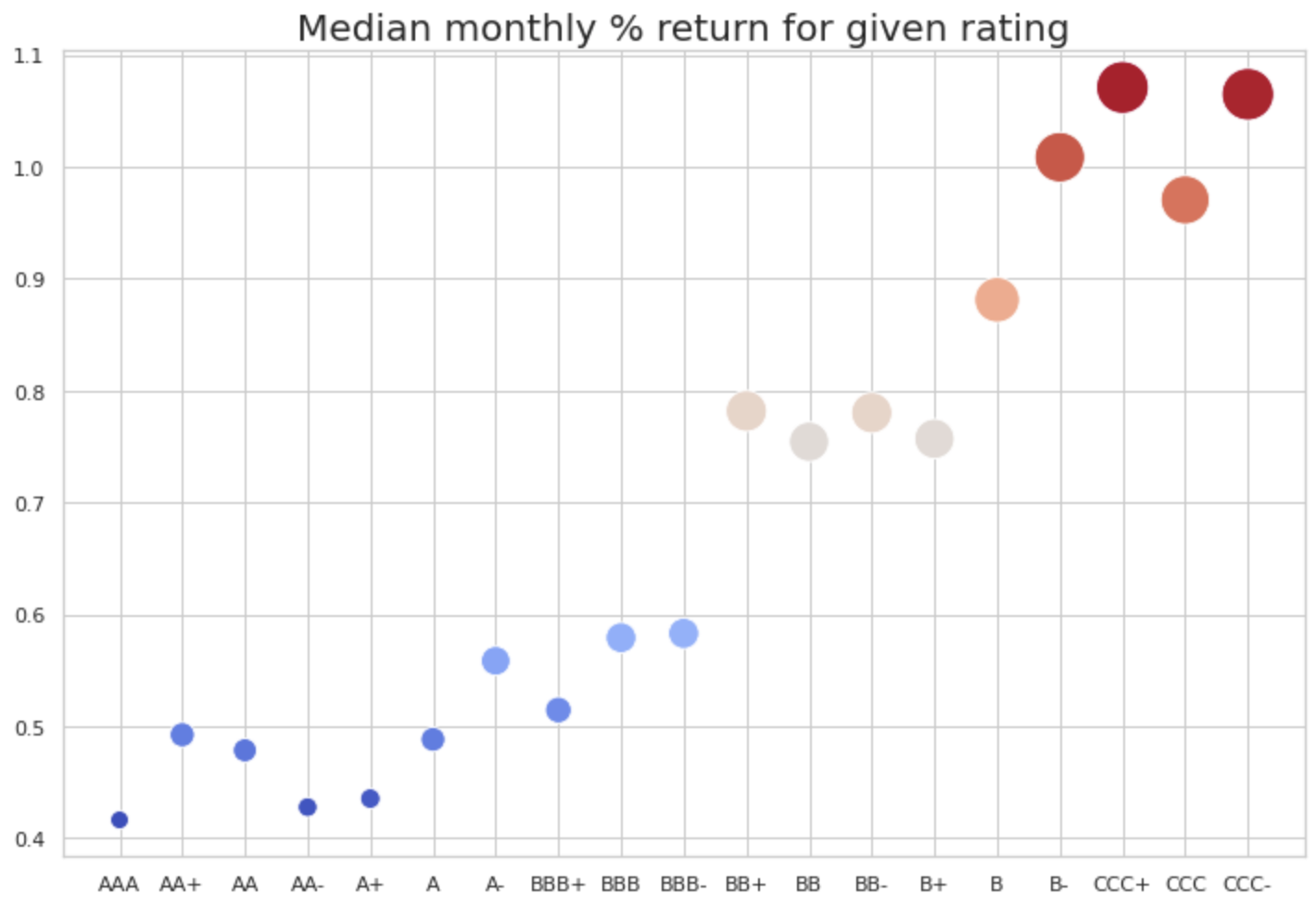
Extending this line of reasoning, it should follow that investors lending money to riskier issuers should expect higher returns on their investment. The empirical evidence supporting this conclusion is overwhelming.
Anecdotally, we show in Figure 1 that this is certainly true for the bonds in our database (We remark that the second chart does not account for survivorship bias. When a bond gets downrated, we simply remove it from the rating category. The bias might make results on the lower end of credit ratings less reliable). Investors holding a broad portfolio of BB-rated corporate bonds between 2003 and 2020 would have earned almost double the cumulative return on a broad portfolio of AA-rated bonds. We created largely diversified portfolios across all other sources of risk, thus attempting to isolate the effect of the default risk factor. We believe that this is enough to motivate a comprehensive analysis of the sources of risk driving the cross section of corporate bond returns.

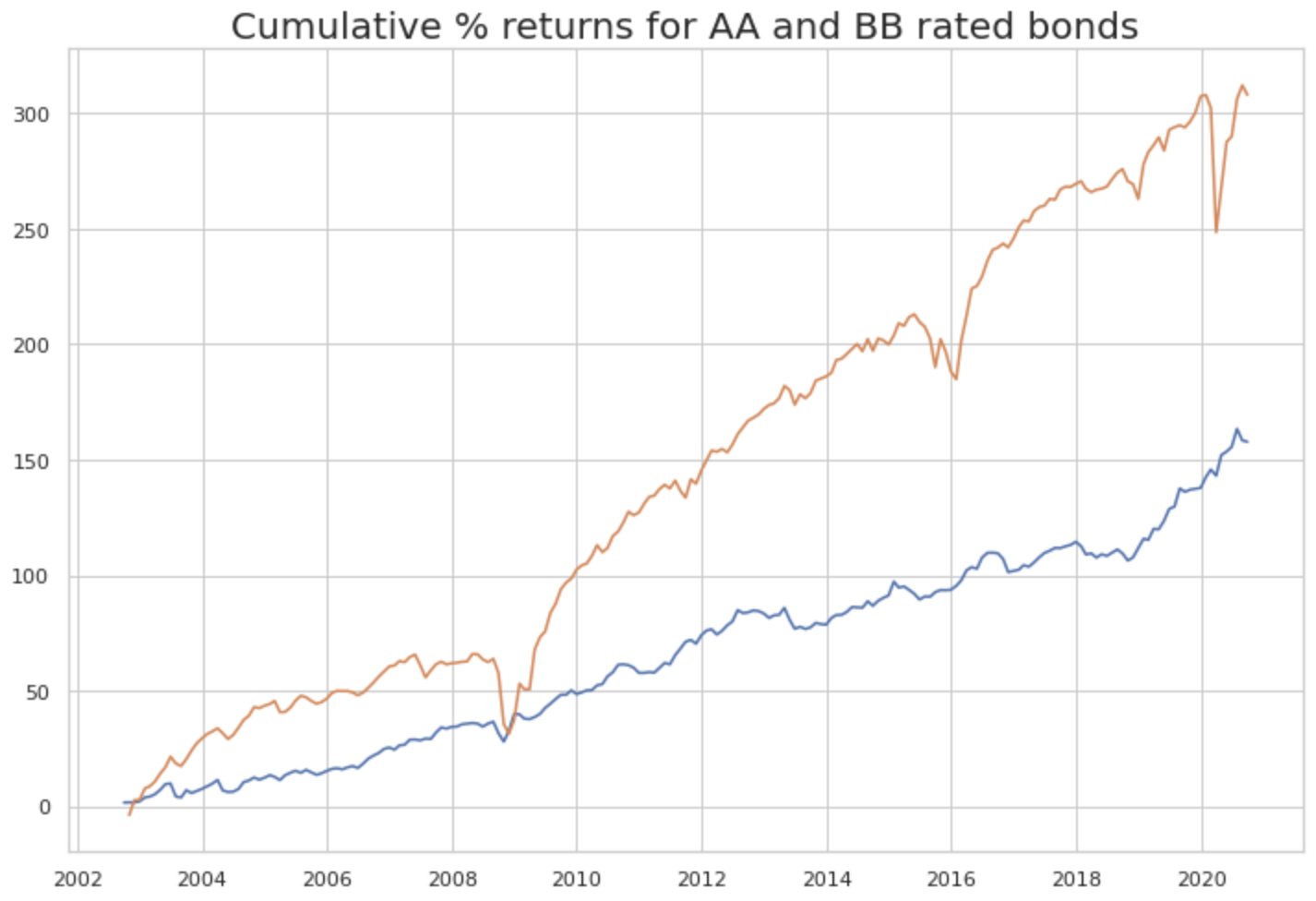
Source: BSIC

We perform a comprehensive cross-sectional analysis where we include a large set of factors: credit risk, value, illiquidity, downside risk and unanticipated shocks to inflation and interest rates. All of our factors are non-traded and constructed with a \say{structural} or theory-based approach. That is most evident in our definition of the value factor and the construction of its proxy. This differentiates our paper from the stream of literature that relies on Fama-French style long-short portfolios to define the factors.

We denote the risk-free rate for maturity $t$ by $r_t^f$ , excess returns for bond $i$ by $\overline{r}_i^e = r_{i,t} - r_{f,t}$ , monthly changes in the value of a variable $x$ by $\Delta x$ . When we refer to an estimate for a coefficient $\beta$ , we write $\hat{\beta}$ . In formulas, we use $Cov$ to refer to the covariance and $\sigma$ to the standard deviation.

Data

We use the WRDS (https://wrds-www.wharton.upenn.edu) Bond Returns database, the Center for Research in Security Prices (https://www.crsp.org, CRSP) Stock / Security Files database (The Center for Research in Security Prices, LLC (CRSP) maintains the most comprehensive collection of security price, return, and volume data for the NYSE, AMEX and NASDAQ stock markets) for some firm characteristics and other pieces of information extracted from equity prices and the TRACE Enhanced (Trade Reporting and Compliance Engine) database for transaction data needed to construct the illiquidty proxy. Finally, we rely heavily on the Bloomberg Terminal and Eikon Refinitiv to complement our databases and add missing data, for instance historical market capitalization data.

The WRDS Bond Database is a cleaned database of US Corporate Bonds. It incorporates two feeds: FINRA’s TRACE, covering over-the-counter corporate bond transactions, and Mergent FISD data for bond issue and issuer characteristics. The available data is of monthly frequency and spans the period from July 2002 to September 2020, covering almost two decades.

Databases of fixed income securities are more difficult to constitute than those focused on equity securities. This is partly due to the over-the-counter nature of bond trading and the consequent lower transparency. However, there is large support in the literature for the use of the the TRACE database, which is found to be reliable due to its use of transaction data.

We took the following steps to further clean the database and ensure the absence of selection bias:

We remove bonds whose offering date is before the start of our database (July 2002).
We remove bonds with embedded optionality, since the latter distorts the return calculation.
We remove subordinate and junior bonds, as they would introduce undesired population heterogeneity in our sample.
We remove bonds maturing in less than one year since they get delisted from major bond indices and, hence, removed from the portfolios of passive investors, creating distortions in the return calculation.
We remove bonds whose monthly dollar trading volume is below $ 10,000 because, as Bessembinder, Maxwell, and Venkataraman 2006 point out, this improves the robustness of the analysis to outliers.
We remove bonds whose maturity is above 30 years, because any bootstrapping methodology makes estimation of yields for longer time horizons entirely arbitrary.
We remove companies for which we have fewer than 72 bond-month observations. We do this because we to compute rolling historical VaR we use 20 months of data, and we need at least 60 additional observations for the computation of factor loadings, as we adhere to the rule of thumb whereby at least 10 observations are needed for each variable in the regression model.

Finally, we are aware that one of the assumptions of linear factor models is the absence of market frictions. We acknowledge that such an assumption might be perceived as unrealistic in the bond market, however, we remark that some of the steps we describe above should have the impact of reducing the impact of friction on the data generation and recording process, making the concern less significant for the purposes of our study.

Methodology

We investigate the cross-sectional relation between corporate bond expected returns and a number of risk factors: credit risk, value, illiquidity, downside risk, unexpected shocks in inflation and unexpected changes in interest rates.
We perform our statistical analysis on excess returns $\overline{r}_i^e = r_{i,t} - r_{f,t}$ , namely bond returns less one-month risk-free rates.

The Fama and MacBeth steps consists of a first pass where we obtain the factor loadings by regressing the time series of returns for each portfolio on the factor proxies:

$\overline{r}_i^e = \alpha_i + \hat{\beta}_{i,DEF} \; DEF_{i,t} + \hat{\beta}_{i,Value} \; Value_{i,t} \hat{\beta}_{i,ILLIQ} \; ILLIQ_{i,t} +$

$+ \hat{\beta}_{i,DOWN} \; DOWN_{i,t} + \hat{\beta}_{i,DxUI} \; DxUI_t + \hat{\beta}_{i,U\Delta IR} \; U\Delta IR_t + \hat{\varepsilon}_{i,t}$

and a second pass where we regress the cross section of expected excess returns for each portfolio onto the factor loadings estimated in the first pass:

$E[\overline{r}_i^e] = \hat{\gamma}_0 + \hat{\gamma}_{DEF} \; \hat{\beta}_{i,DEF} + \hat{\gamma}_{Value} \; \hat{\beta}_{i,Value} + \hat{\gamma}_{ILLIQ} \; \hat{\beta}_{i,ILLIQ} + \\ + \hat{\gamma}_{DOWN} \; \hat{\beta}_{i,DOWN} + \hat{\gamma}_{DxUI} \; \hat{\beta}_{i,DxUI} + \hat{\gamma}_{U\Delta IR} \; \hat{\beta}_{i,U\Delta IR} + \hat{\nu}_i$

thus estimating the vector of risk premia as coefficients:

$\hat{\boldsymbol{\gamma}}'=[\hat{\gamma}_0 \; \; \hat{\gamma}_{DEF} \; \; \hat{\gamma}_{Value} \; \; \hat{\gamma}_{ILLIQ} \; \; \hat{\gamma}_{DOWN} \; \; \hat{\gamma}_{DxUI} \; \; \hat{\gamma}_{U\Delta IR}]$

Differently from Fama and French 1993 and most other papers in the literature, we do not construct long-short portfolios that seek to have beta equal to one for the factor exposure they intend to isolate and zero loading for all other factors.
It has been pointed out in several papers that constructing such long-short portfolios is not always practical or even viable with corporate bonds. Even if it were always possible, transaction costs to short many corporate bonds are often high and thus the theoretical return obtain through statistical construction would not reflect real returns earned if the strategy were to be implemented and would inflate the upside.

Houweling and Zundert 2017 [16] address this issue by constructing long-only portfolios applying the overlapping portfolio methodology in Jegadeesh and Titman 1993 [17]. We prefer to use non-traded proxies to construct the factors, and we discuss our proxy construction methodology in great detail in Section ??. Using the Fama-Macbeth 1973 two-pass regression allows us to extract factor risk premia without using traded factors.

We conduct separate analyses for IG and HY bonds, because empirical evidence shows that those two corporate bond market segments are treated by investors essentially as two different asset classes. While index providers and asset managers might offer both IG and HY portfolios and funds, those are generally addressed to different types of clients and investors which are heterogeneous in risk appetite, portfolio mandate, investment goals, and regulatory constraints.

This market segmentation has been studied and documented for instance in Ambastha
et al. 2010 [18] and Z. Chen et al. 2014 [19]

Finally, we need to perform some sort of portfolio sorting, since for some bonds we do not have enough observations to perform factor loading estimation without running out of degrees of freedom (especially for high yield bonds). The sorting scheme we decide to adopt is by company, namely we create a bond portfolio for each company for which we have securities in our databases.

Constructing the proxies

We now discuss the factors we include in our cross-sectional analysis and the proxies we construct to measure exposure to those factors. Due to lack of access to certain pieces of data, we do not include the size factor in our analysis. This is quite unfortunate due to the significant amount of evidence that has been put forward for its relevance (see Zundert 2017, Israel, Palhares, and Richardson 2017, Bektic et al. 2016).

For the interest of the reader, we remark that in the corporate bond space, an analysis of the significance of the size factor in the cross section of returns is performed by proxying for size through total debt outstanding. This is different from equities, where size is measured as the market capitalization of the company.

Incidentally, Bektic et al. 2016 use market capitalization to measure the size factor in bond returns, and they motivate their choice with reference to Merton 1974, which links default risk to the company’s capital structure (Bektic et al. 2016 motivate their choice arguing that ” in the tradition of Merton 1974, changes in equity and corporate bond prices should be related as they represent claims against the assets of the same company […]. For instance, if the equity price increases to incorporate positive news, the probability of default decreases and this should affect the bond price positively, and vice versa. The correlation in this relationship suggests, that any factor which has predictive power for equity returns is in principle an eligible candidate to forecast corporate bond returns as well due to the no-arbitrage principle).

We believe that total debt outstanding is a more direct measure of the risk entailed in exposure to the size factor when analyzing the cross section of corporate bonds, hence, its use should reduce noise and measurement error.

Credit Risk

To proxy for default risk, we rely on the insights in Merton 1974 and Fama and French 1993.

The Merton Model estimates the probability of default by comparing a firm’s value to the face value of its debt. Since the market value of a levered firm is not observable, the Merton model infers it from the market value of the firm’s equity. If the firm’s debt is treated as a single zero-coupon bond with maturity $T$ , then equity can be thought of as a call option on the firm value with a strike price equal to the firm’s debt.

As an example, we can consider a firm at maturity: if the firm’s value is below the face value of debt, then the equity holders will walk away and let the firm default; but if the firm value exceeds the face value of debt, then the equity holders will want to exercise the option and collect the difference between firm value and debt.

More formally, the equity value can be represented by the Black-Scholes option pricing equation (see Black and Scholes 1973, Merton 1973). When the volatility of equity is considered constant within the time period $T$ , the equity value is:

$E(V,t) = V \mathcal{N}(d_1)- e^{-rt} D\mathcal{N}(d_2)$

where $V$ is firm value, $t$ is duration, $E$ is equity value as a function of firm value and time duration, $r$ is the risk-free rate for the duration $t$ , $D$ is the value of debt, $\mathcal{N}$ is the cumulative normal distribution, and $d_1$ and $d_2$ are defined as in a standard European call option:

$d_1 = \frac{\log \frac{V}{D}+ (r_t^f + \frac{1}{2} \sigma^2_V ) \ t}{ \sigma_V \ \sqrt{t}}$

$d_2 = d_1 - \sigma_V \sqrt{t}$

while the volatility of equity will be:

$\sigma_E = \sigma_V\ \frac{V}{E}\ \mathcal{N}(d_1)$

From this point, a solver will be instrumental to infer the precise value of $V$ and $\sigma_V$ . As a last step, the Distance to Default and the Probability of Default of a given company, with a typical $t = 1$ year horizon, are given by

$\text{DD} = \frac{\log \frac{V}{B}+ (\mu + \frac{1}{2} \sigma^2_V ) \ t}{ \sigma_V \ \sqrt{t}}$

$\text{Probability of Default} = \mathcal{N} (-\text{DD})$

Notably, the model assumes that the firm’s value $V$ follows a Geometric Brownian motion from a specific point in time $t$ to $t+1$ , and the probability of lying withing the default area will follow a Normal Distribution.

To this day, the Merton model is overwhelmingly used by credit agencies, with its refinement known as the Merton’s KMV – where a different structure of the company’s liabilities and the empirical distribution of its returns are used.

Value

We adopt the definition of the fixed income value factor found in Shen, Pathammavong, and A. Chen 2019: “the value factor in fixed income cannot directly borrow the definition from equity, and cannot be purely fundamental driven. Nonetheless, it can take the same philosophy from the equity value factor, that is, to identify the relatively undervalued securities or, more specifically, to evaluate the relative cheapness compared with the underlying riskiness. […] we define value as the difference between the market-priced credit spread and the model-implied credit spread of individual bonds”. The value factor is constructed as the spread between the market value of the option-adjusted spread (OAS) and a model-implied value of the same. Notably, in the absence of embedded optionality, the OAS reduces to the Z-spread, and since we exclude convertibles and other embedded-optionality bonds from our sample, we can employ the Z-spread directly.

The Z-spread is the constant spread that, added to the risk-free rate, discounts all future coupons and principal repayment to obtain the price of the bond, according to the following formula (considering a bond that pays annual coupons for simplicity):

$P = \frac{c}{(1+r_1^f + Z^{mkt})} + \frac{c}{(1+r_2^f + Z^{mkt})^2} + \ldots + \frac{FV}{(1+r_N^f + Z^{mkt})^N}$

essentially representing a parallel shift over the yield curve. We compute the market-value Z spread $Z^{mkt}$ for each bond-month observation using a proprietary model we constructed in Python that relies on the Newton method via scipy.optimize.

We construct the model implied Z-spread by performing the following regression:

$Z_{i,j} = \sum_{k=1}^n \beta_{k,j} u_{i,k} +\gamma_{1, j} T_i + \gamma_{2,j} T_i^2 + \varepsilon_i$

Here, $j$ represents the various industries for the database, $k$ a group of credit ratings and $T$ the time to maturity of each bond.
The double dummy is included to reflect the logically different credit spreads between bonds of different ratings and industries. The quadratic term, on the other hand, contributes to the model by adding curvature, as the difference between short-term and medium-term bonds cannot be compared with the one between medium-term and longer-term bonds.

Finally, we obtain our value factor proxy as

$Value_t = Z_{i,t}^{mkt} - Z_{i,j}$

where $i$ identifies the bond, $t$ the month and $j$ the industry.

Shen, Pathammavong, and A. Chen 2019 find that the fixed income value factor, just like the equity equivalent, is highly cyclical, performing better during recovery and expansion phases. Several explanations have been put forward in the literature for the existence of a value premium, ranging from behavioral to financial origins. Particularly troublesome from the point of view of market efficiency is why certain companies (in the case of equities) or securities (in the case of fixed income) remain undervalued for prolonged periods. All the same, the essence of the value factor is that cheaper securities should outperform \textit{richer} ones.

Illiquidity

The importance of the illiquidity factor in the cross section of corporate bonds is well documented in the literature (Lin, Junbo Wang, and Wu 2011, Bao, Pan, and Jiang Wang 2011, Bai, T. G. Bali, and Wen 2019). In fact, liquidity (or lack thereof) was one of the first factors to be considered in pricing the cross section of corporate bond returns alongside default risk.

To proxy for illiquidity, we choose to follow the approach in Bao, Pan, and Jiang Wang 2011, as much of the literature does. The authors assume that the log price $p_t$ consists of a fundamental and a transitory component:

$p_t = f_t + u_t$

where $f_t$ follows a random walk and the magnitude of $u_t$ represents the impact of illiquidity.
Then, given the change in log prices, $\Delta p_{it} = p_{it} - p_{it - 1}$ , the illiquidity factor is given by

$ILLIQ = - Cov_t (\Delta p_{it}, \Delta p_{it + 1})$

since, under the random walk assumption for $f_t$ , $ILLIQ$ isolates the impact of the transitory component $u_t$ .

We compute the monthly value for the illiquidity factor using daily prices in the TRACE dataset. It is essential to use transaction datasets to compute such a proxy, and TRACE contains almost 300 million trade records for the bonds we consider. What is more, the significance of the illiquidity factor decreases when computed with weekly or, even worse, monthly data, hence our use of daily data is justified by the expectation of statistical robustness.

To assess the reliability of this proxy to measure the illiquidity risk factor, we also use the dollar monthly trading volume as an alternative and check if our coefficient is more significant and/or of different magnitude.

Downside Risk

Bondholders are much more sensitive to downside risk than stockholders. That is because, as Bai, T. G. Bali, and Wen 2019 point out, bondholders receive cash flows equal to the fixed coupons and principal payment at maturity, thus not benefiting form positive news on firm fundamentals. This is essentially a cap on the upside, resulting in bond returns being concave in investor beliefs about the underlying fundamentals. Equity returns, on the other hand, should be linear in fundamental beliefs.
Hence our persuasion in the importance of including downside risk in our analysis of the cross section of credit returns.

We proxy for downside risk through the monthly Value at Risk (VaR), which shows how much the price can go down with a given probability. We consider the non-parametric approach that uses actual historical data of bond returns. For its computation, we include company-level portfolios with at least 80 observations and select the second-smallest (using the smallest would drastically reduce variability in the proxy. Hence, we use the second smallest) observation of a 20-month rolling window to compute the 10\% VaR. This unconventional measure is employed to ensure there are at least 60 data points to run the regression and thus estimate factor loadings.

Macro

On a macroeconomic level, we evaluate the impact of exposure to unexpected changes in inflation and interest rates.

In efficient markets, anticipated changes in inflation and interest rates cannot represent a risk exposure or command a risk premium in terms of expected returns, because rational investors incorporate available information in prices. On the other hand, the possibility that inflation and interest rates will change unexpectedly due to unforeseen circumstances requires to be treated as a separate source of risk in the cross-sectional analysis of corporate bond returns. Firstly, such risks are unrelated to the other factors listed above, hence satisfying the full rank requirement of the factor matrix. Secondly, bond prices are directly affected by interest rate and inflation risk, so that the two could be defined as \textit{structural} risk exposures for bonds. Both inflation and interest rates contribute to defining the factor by which future cash flows are discounted. If we consider that linear factor models can be seen as a way to estimate the stochastic discount factor, our analysis would be lacking if macro sources of risk were dismissed.

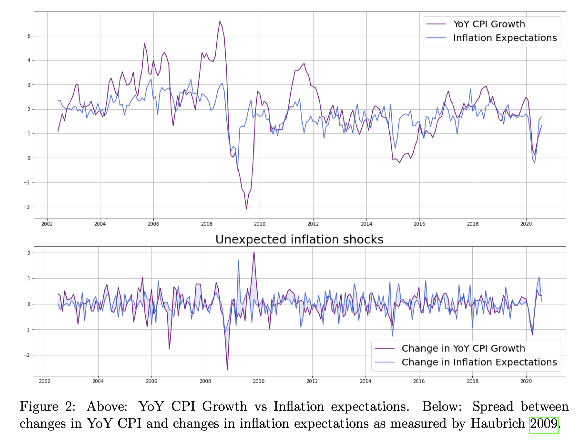
As far as inflation is concerned, we propose an original proxy which we call $\text{Duration times Unanticipated Inflation}$ (DxUI). Our proxy is defined as:

$DxUI_t = \frac{\partial P}{\partial y} \times UI_t$

$UI_t = (\Delta CPI_t - \Delta 1YEI_t)$

where $1YEI_t$ is our label for the one-year forward inflation expectation index provided by the Federal Reserve Bank of Cleveland.
Our data for monthly YoY CPI prints comes from FRED Graph Observations – Federal Reserve Economic Data (https://fred.stlouisfed.org). A visualization of 17 is shown in Figure 2.

We decide to construct our proxy for unanticipated inflation as in the first expression above, as opposed to using the second, because we consider that bonds with different duration are impacted by inflation risk in different ways. For instance, a 30 year bond is sensitive to the rate of change in the price level over the next 30 years, whereas the real value of the cash flows of a 5-year bond is exposed to such changes only over the 5-year horizon. Hence, inspired by the Duration Times Spread metric of Dor et al. 2007, we decided to weigh the second equation by duration, obtaining the interaction term of the first equation.

We believe our findings on the risk premium for exposure to inflation risk are an important contribution to the existing literature, which does little to shed light on the existence and magnitude of an inflation risk premium in corporate bond returns. Most notably, Kang and Pflueger 2015 research the relation between inflation uncertainty and credit spreads (Kang and Pflueger 2015 argue that “Inflation risk can increase credit spreads in two ways. First, more volatile inflation increases the ex ante probability that firms will default due to high real liabilities. Second, when inflation and real cash flows are highly correlated, low real cash flows and high real liabilities tend to hit firms at the same time, increasing default rates and real investor losses. In this second case, higher credit spreads reflect higher expected credit losses and a higher risk premium due to the greater concentration of defaults in high marginal utility states”). If Kang and Pflueger 2015’s findings are robust and higher inflation uncertainty does lead to higher bond spreads, we should expect that volatility in the rate of change in prices also leads to higher returns, insomuch as it represents a risk factor that bond investors accept exposure to. While we do not include inflation volatility in our analysis, we do include unanticipated changes in inflation, and we should expect for them to have a positive significance in driving returns inasmuch as unanticipated changes should be thought of as volatility enhancing.

Source: Kang and Pflueger 2015

Moving to unanticipated changes in interest rates, we construct our proxy by modeling changes in the risk-free rate as a linear function of changes in expected interest rates. Clearly, interest rate expectations are not directly observable, hence we need an instrumental variable. We choose to use forward rates as an instrument for expectation. An instrument needs to satisfy three validity conditions:

Exogeneity, i.e., $Cov(IV_t, \eta_t) = 0$ ,
Relevance,
Exclusion restriction.

The third condition requires that the instrument not affect the dependent variable (changes in risk-free rate) other than through the variable it instruments (expectations of future interest rates).

Evidence for condition 2 can be found in Fama 1976, Fama and Bliss 1987, and Svensson 1994.
A case could be made that, given the low $R^2$ of the regression below ( $R^2=0.103$ ), there is a lot of unexplained variability in the form of omitted variables. If those variables are not orthogonal to the instrument, the covariance between the instrument and the error term would be different from zero and the estimated coefficients would be inconsistent.

Our response is that, from a “structural” point of view, the main explanatory factors for short-term risk-free rates that could be covariates of our instrument are the central bank policy rate and in general monetary policy. However, through forward guidance, credible and independent central banks such as the Federal Reserve can shape expectations of future interest rates, hence it is sensible to assume that after controlling for those expectations, policy variables would have insignificant loadings, hence not leading to omitted variable bias.

We thus extract the expected component of changes in the risk-free rate and residualize the unexpected component:

$\hat{\eta}_t = \Delta {r}_t^f - \hat{\beta}_0 - \hat{\beta}_{fwd} \; \Delta E[r_{t+1}^f]$

$\text{IV:} \quad \Delta E[r_{t+1}^f] = \Delta r_{t}^{1y \; fwd}$

For the computation of forward rates we rely on the model in Gurkaynak, Sack, and Wright 2010 and the data they provide. We choose to use the 1-year maturity for both Treasuries and forward rates (1-year rate starting 1 year hence) because long-term rates are affected by 1. expectations about future short term rates, 2. a term premium, 3. an inflation risk premium, and 4. potential uncertainty premia. We want to avoid exposure to those components, as they would introduce measurement error, hence we choose to use short-term rates, which are primarily driven by monetary policy, and short-term forward rates, which shouldn’t incorporate any significant term premium and inflation premium.

A visualization of the residuals is shown in Figure 3.

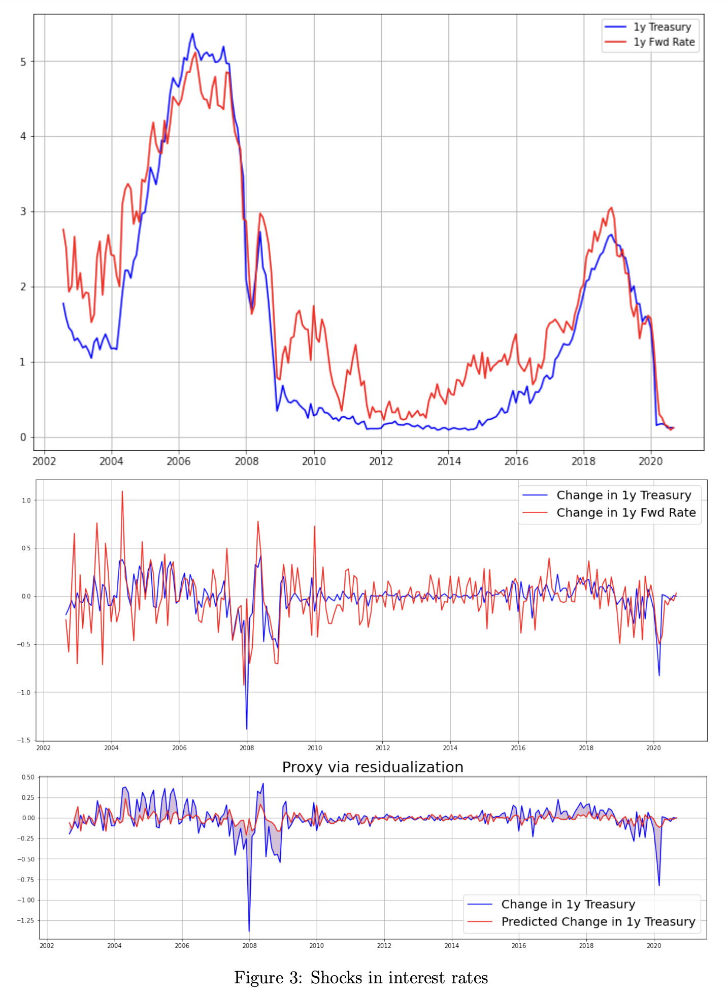
Source: Gurkaynak, Sack, and Wright 2010

Summary Statistics and Analytics

We begin by performing the Jarque-Bera normality test on the return series for the bonds in the database, separating IG from HY. For each bond, we compute the p-values of the tests, and we plot their cumulative density alongside the 0.05 threshold. From the graphs in Figure 4 we learn that for a bit over half of the IG bonds we do not find sufficient evidence to reject the normality hypothesis. For HY bonds, on the other hand, that amount reduces to close to 20%.

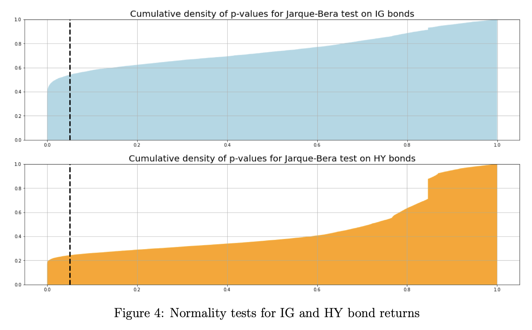
Source: BSIC

However, it might be the case that our results are biased by the small number of return observations for several bonds in the two datasets (due to illiquidity and other issues). To address this concern, we decide to select for each credit rating the bond with the longest return time series available in our data and we use is as a representative bond to test for normality of returns. The results are displayed below.

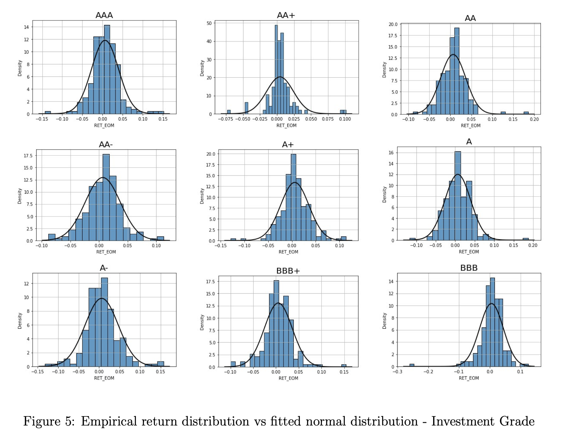
Source: BSIC

References

[1] Ambastha, Madhur et al. (2010). “Empirical Duration of Corporate Bonds and Credit Market Segmentation”. In: The Journal of Fixed Income 20.1, pp. 5–27.

[2] Bai, Jennie, Turan G. Bali, and Quan Wen (2019). “Common risk factors in the cross-section of corporate bond returns”. In: Journal of Financial Economics 131.3, pp. 619–642.

[3] Bali, Turan, Robert Engle, and Scott Murray (Aug. 2017). Empirical Asset Pricing: The Cross Section of Stock Returns: An Overview. isbn: 9781118445112.

[4] Bao, Jack, Jun Pan, and Jiang Wang (June 2011). “The Illiquidity of Corporate Bonds”. In: Journal of Finance 66, pp. 911–946.

[5] Bektic, Demir et al. (Jan. 2016). “Extending Fama-French Factors to Corporate Bond Markets”. In: SSRN Electronic Journal.

[6] Bessembinder, Hendrik, William Maxwell, and Kumar Venkataraman (2006). “Market transparency, liquidity externalities, and institutional trading costs in corporate bonds”. In: Journal of Financial Economics 82.2, pp. 251–288.

[7] Black, Fischer and Myron S Scholes (May 1973). “The Pricing of Options and Corporate Liabilities”. In: Journal of Political Economy 81.3, pp. 637–654.

[8] Campbell, John Y. (2018). Financial Decisions and Markets: A Course in Asset Pricing. Princeton University Press.

[9] Chen, Nai-fu (1983). “Some Empirical Tests of the Theory of Arbitrage Pricing”. In: Journal of Finance 38.5, pp. 1393–1414.

[10] Chen, Zhihua et al. (2014). “Rating-Based Investment Practices and Bond Market Segmentation”. In: Review of Asset Pricing Studies 4.2, pp. 162–205.

[11] Cochrane, John H. (2005). Asset Pricing: Revised Edition. Princeton University Press. isbn: 9780691121376.

[12] Dor, Arik Ben et al. (2007). “Duration Times Spread”. In: Journal of Portfolio Management.

[13] Fama, Eugene F. (1976). “Forward rates as predictors of future spot rates”. In: Journal of Financial Economics 3.4, pp. 361–377.

[14] Fama, Eugene F. and Robert R. Bliss (1987). “The Information in Long-Maturity Forward Rates”. In: American Economic Review 77.4, pp. 680–92.

[15] Fama, Eugene F. and Kenneth R. French (Feb. 1993). “Common risk factors in the returns on stocks and bonds”. In: Journal of Financial Economics 33.1, pp. 3–56.

[16] Fama, Eugene F. and James D. MacBeth (May 1973). “Risk, Return, and Equilibrium: Empirical Tests”. In: Journal of Political Economy 81.3, pp. 607–636.

Published by BSIC on 10 April 202210 April 2022

0 Comments

Leave a Reply Cancel reply

Markets

Japan, 30 years of economic failure: have we finally come to a reflationary turn?

Markets

Market Recap 14/04/2024

Markets

Feature Selection and Engineering for Time Series Data

WHAT DRIVES CREDIT? Understanding the Cross Section of Expected Corporate Bond Returns

Published by BSIC on 10 April 202210 April 2022

0 Comments

Leave a Reply Cancel reply

Related Posts

Markets

Japan, 30 years of economic failure: have we finally come to a reflationary turn?

Markets

Market Recap 14/04/2024

Markets

Feature Selection and Engineering for Time Series Data