Commodity futures have become a widespread vehicle amongst investors and traders as they can be used for strategic and tactical asset allocation. The strategic appeal of commodity indices comes from the equity-like return, their key diversification role, and their inflation-hedging properties.
The term structure of commodities usually refers to the difference between future prices of different maturities at a given time point. It is essential for commodity hedgers and speculators to know the shape of the futures curve as it serves as a forecast of future spot prices. Furthermore, this information is very useful for managers of companies in the commodities space. Adjusting stock levels, production rates, hedging exposures, and many more parameters hinge on such information.
While, in the short-term, commodities markets are highly affected by microstructural events within the realms of the industry, they operate in a global economy driven by interest rates and economic activity. Especially now, with highly volatile interest rates at elevated levels compared to previous decades, it is worth understanding how interest rates may affect their price action.
Thus, in this article, we give economic intuition for constructing the term structure of commodity futures, how these may be affected by interest rates, and finally have a look at some empirical evidence in the literature, trying to replicate it ourselves.
Term Structure of Commodities
Keynes (1930) and Cootner (1960) proposed the idea that commodity futures prices depend on the net position of hedgers. This can be interpreted as a form of insurance: producers and consumers of the underlying commodity transfer the risk of price fluctuations to speculators, which are willing to undertake this risk for future expected positive returns.
The term structure of commodities can have two forms. Firstly, the increase in the future prices as maturity approaches is known as normal backwardation, and secondly, the decrease in the futures price as maturity approaches is referred to as contango. Both contango and normal backwardation arise because of the inequality between the long and short positions of hedgers, which require the intervention of speculators to restore equilibrium. Therefore, commodity futures prices are directly related to the propensity of hedgers to be net long or net short.
Contango refers to a situation where the futures price of an underlying commodity is higher than its current spot price, it means that the market expects that the price of the underlying commodity will rise in the future and as such, market participants are willing to pay a premium for it now. As the maturity date approaches, it is always observed that the forward price in contango converges downwards towards the commodity’s future spot price. The opposite is observed in backwardation, where at maturity, the forward price will converge upwards towards the expected future spot price.
Interestingly, the known arbitrage condition that determines the relationship between spot and futures prices for any financial asset rarely holds for commodities. The intricate and dynamic connection between spot and future prices is shaped by various factors, including the function of commodities as items for consumption and processing, as well as the crucial significance of physical inventories. Within the commodity market, there are some imperfections that influence the forward and spot price behaviour and inhibit arbitrage. Arbitrage is impossible if the commodity cannot be stored, such as electricity. Arbitrage can be further slowed down by difficulties associated with the localization of the delivery points of the futures contracts of the commodity.
The commodity curve is mostly influenced by four factors:
1. Funding and storage costs
As for funding costs, it is easy to see how higher interest rates affect funding costs adversely, making it more expensive to hold a stock of commodities. This dynamic often results in a steeper contango because holding it today is less desirable than in the future since you can avoid the cost by entering the futures contract.
As for storage costs, they vary widely amongst the different commodities since there are many types of storage costs:
a. Warehousing Fees: Charges for renting or maintaining space where the commodity is stored. A higher cost of capital stemming from elevated interest rates may lead to higher leasing costs for warehousing these commodities so landlords can break even. However, if higher interest rates cause lower economic activity in the given commodities vertical – many of which are highly sensitive to macroeconomic conditions – then lower demand may give stronger bargaining rights for tenants, thereby lowering warehousing fees.
b. Insurance Costs: Premiums paid to insure the commodity against risks like theft, damage, or loss during storage. The insurance costs can be substantial, especially for high-value commodities like precious metals, which are not only expensive but also have a high risk of theft due to their easy convertibility into cash. It is unclear what effects interest rates have – it is highly dependent on the structure of such insurance contracts as well as the insurer’s portfolio; higher rates may mean greater investment income, allowing insurers to offer more competitive rates. However, lower asset values may lead to the opposite conclusion.
c. Security Costs: Expenses for security measures to protect the commodity. They include surveillance systems, guards, and other security protocols, especially critical for commodities like oil and gas, which face risks of spills, environmental damage, and explosions.
d. Handling and Maintenance Costs: These costs are associated with moving, managing, and maintaining the quality of the commodity during storage. They are particularly significant for sensitive or perishable items like agricultural commodities.
e. Deterioration or Obsolescence Costs: Some commodities may incur costs related to deterioration over time or obsolescence, especially in rapidly changing markets. This is particularly relevant for agricultural commodities, which can spoil or lose value over time.
Overall, storage and funding costs are affected by a myriad of factors, but on a larger scale may have a substantial effect on the cost of carry of a commodity, thereby affecting its futures curve.
2. Convenience yields
On the opposite end of the spectrum, convenience yields are benefits one accrues from holding a commodity. Because the presence of a convenience yield (in the absence of any costs) means that you make money today from holding a commodity, this results in backwardation, or a flatter shape of the term structure of the commodities future curve, where futures prices are below those of spot prices.
The most prominent example of when convenience yield kicks in is during a shortage when the spot price of a commodity is oftentimes higher than the futures price. Although one could try to make a connection between interest rates and convenience yields, these may be second or third-order effects which usually have much lower significance than the microstructural factors at play.
3. Hedging pressures
Usually, commodities producers are bigger hedgers of the commodities than the consumers since commodities prices are usually one of many input prices, whereas most commodities production firms’ revenues are directly correlated to the price of the commodity. Therefore, hedging pressures are usually to the downside, contributing to a flatter curve.
4. Expected supply-demand imbalances
Supply-demand imbalances in commodity markets, influenced by factors like financialization, interest rates, supply shocks, and seasonality, play a crucial role in shaping market dynamics and pricing structures. With the increased financialization of the past decades, including making investments in asset classes that were previously inaccessible to retail investors like commodities, an influx of long-only demand has emerged. However, these rate-sensitive flows can counter this trend when interest rates go up.
Supply imbalances, especially sudden shocks due to geopolitical events or natural disasters, can cause significant disruptions. These shocks can lead to immediate shortages, pushing spot prices higher and often resulting in a state of backwardation, even for commodities that are usually in contango like oil.
Additionally, seasonality plays a pivotal role in commodities, especially in the agricultural and energy sectors. Seasonal variations in production, such as harvest periods for crops or heating demands in winter, can lead to predictable fluctuations in supply and demand. These seasonal factors are often anticipated by market participants but can still lead to periods of tight supply or excess, impacting prices and market structures.
Commodities and the Yield Curve
The yield curve, historically viewed as a barometer for economic fluctuations, encapsulates a wealth of information about impending economic conditions. It is the shape of this curve—illustrating yields across various maturities of government bonds—that often hints at future economic expansions or contractions. The curve’s predictive prowess stems from market anticipations: a flattening yield curve traditionally forewarns of an economic downturn, whereas a steepening curve signals prospective periods of economic growth. This dynamic is largely due to monetary policy actions, such as the Federal Reserve raising rates to temper inflation, which, in turn, moderates consumption and investment, leading to an economic slowdown followed by revival with lower rates. Consequently, the long-term rates ascend at a slower pace than short-term rates, resulting in a flattening of the yield curve, and vice versa.
Given that commodity prices are tightly interwoven with business cycles, a pertinent inquiry emerges: Can the structure of the yield curve serve as a forecaster for future commodity price movements? This question is of significant interest to investors and policymakers alike, as it explores the potential of the yield curve to predict not just broad economic trends but specific market behaviors. The shape of the yield curve, reflecting the market’s collective expectations about the future, may hold key insights into the directional movements of commodity prices, which are sensitive to economic changes. Commodities, being fundamental to industrial and economic activities, often respond to the shifts in economic outlook that the yield curve suggests.
The research of Yasmeen Idilbi-Bayaa and Mahmoud Qadan (2021) indicates that the yield curve’s forecasting success for monthly commodity price changes was significant from 1986 to the early 2000s. Their estimation results of future returns with the spread between 10 year bonds and 3 month T-Bills shows significant results for multiple commodities. The commodities most affected by yield curve changes were silver and zinc where just these changes explained more than 10% of the variance (R2 were 0.114 and 0.26 respectively) for a 4 quarter ahead forecast with a positive slope of the linear model. So before the beginning of the 2000s, a flattening of the yield curve was an indicator of future price decreases and the other way around. The findings highlight a period where a flattening of the yield curve, characterized by a decreasing spread between long and short-term interest rates, served as a harbinger of falling commodity prices. Conversely, a steepening curve signaled rising prices, illustrating the yield curve’s predictive power in the commodities market. This period demonstrated a clear interconnection between bond markets and commodity pricing, emphasizing the yield curve as a crucial tool for investors and analysts.
Heightened sensitivity in commodities like silver, zinc or natural gas can be partially explained by the hedging activities that are happening in the market. Different commodities attract different hedging strategies by producers and consumers. For commodities with more volatile prices, like silver, hedging activities might be more pronounced, making their prices more sensitive to changes in economic indicators like the yield curve. Interestingly, oil is the only commodity among the observed that shows a different relationship with the linear regression having a negative slope indicating that yield curve steepening suggests a possible future price decrease of oil. In the figure below you can see how 2-year yield decreases holding other factors constant result in the decline in oil prices. This might due to the fact that the oil industry is capital-intensive, requiring significant investment in exploration, drilling, and infrastructure and the smallest decline in interest rates decrease the costs significantly.
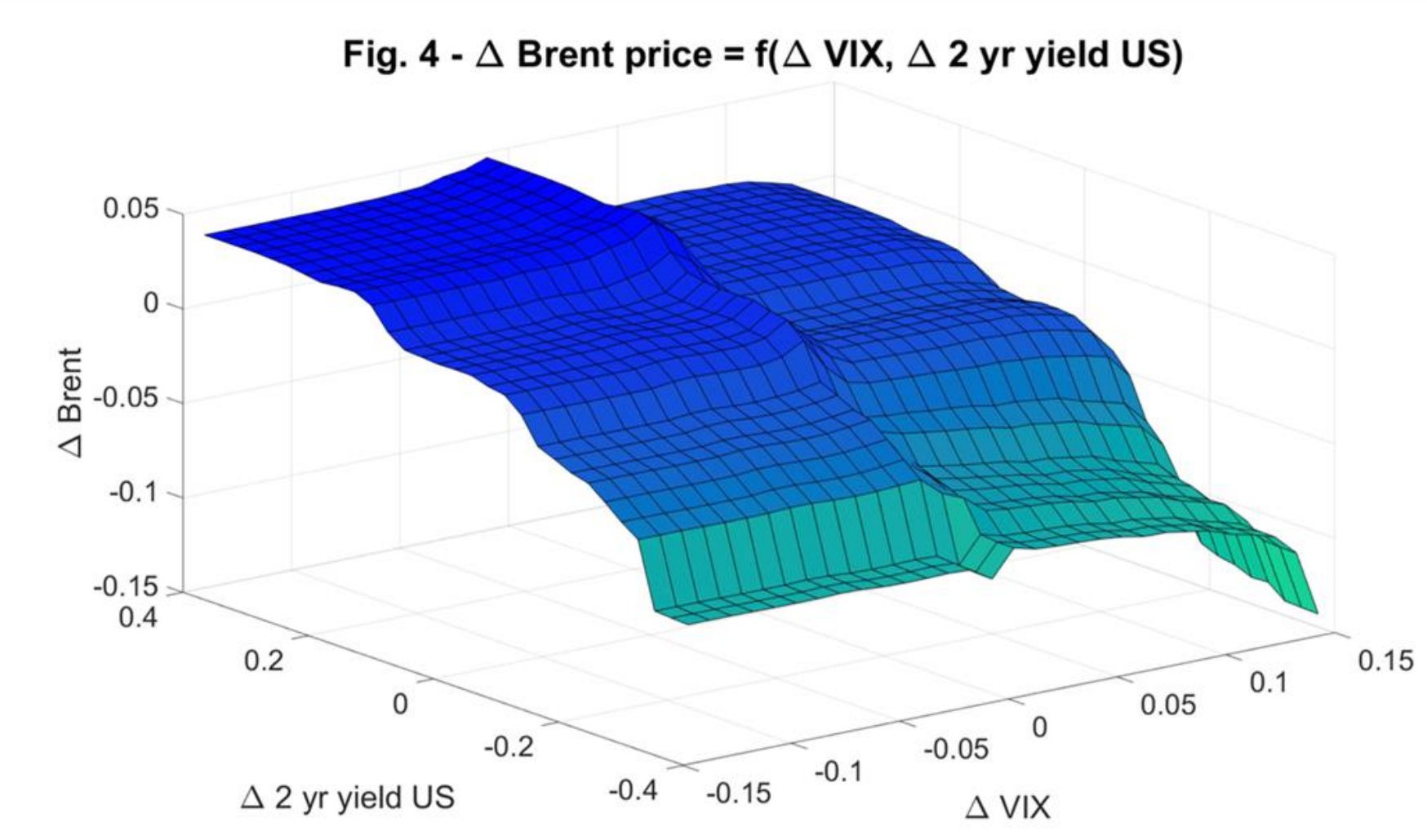
Source: Quantifying the role of interest rates, the Dollar and Covid in oil prices (Kohlscheen 2022)
However, in the period post-2000, the effectiveness of the yield curve as a predictor for commodity prices showed a notable decline. This change can be attributed to increased capital inflows into the commodities market, which in turn fostered a stronger correlation with equity markets. Such developments led to a disruption in the traditional link between commodities and economic cycles, previously observed and relied upon by market analysts and investors. When regressing commodity prices against the yield spread during this period, the results were markedly different, with the explained variance in commodity prices by the yield curve nearing zero.
This shift suggests a significant transformation in the dynamics of financial markets, where commodities began to behave more like financial assets, closely mirroring the trends and movements of equity markets. This change in correlation dynamics indicates a new era in the commodities market, one where the influence of broader financial market sentiments and global capital flows became more pronounced.
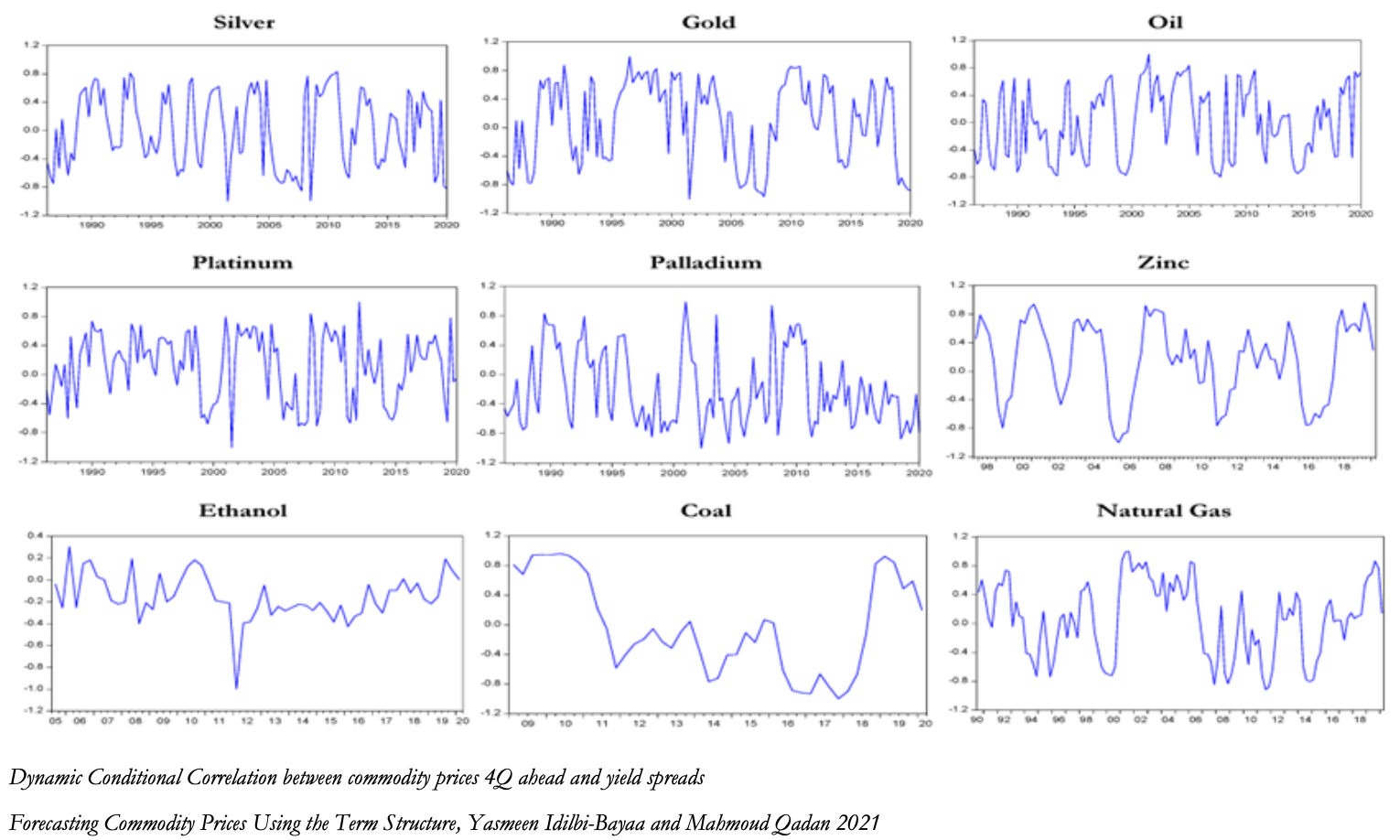
The researchers highlight the unstable nature of the dynamic correlation between the yield curve and commodity prices two, three and four quarters ahead, over time. Their findings point out that this relationship has experienced periods of both positive and negative correlation, indicating that the interplay between these economic indicators is not fixed but rather subject to shifts influenced by varying market conditions. Our own findings confirm these results. To save the reader from comparing multiple graphs we will include our estimates of dynamic correlation for gold prices 4Q ahead and the yield spread between 10-year bonds and 3-month T-Bills.
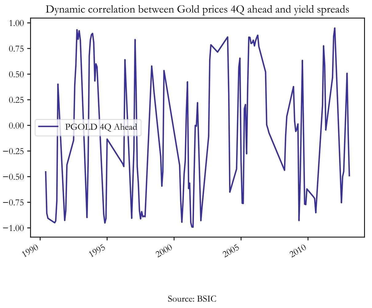
Source: Forecasting Commodity Prices Using the Term Structure (Yasmeen and Mahmoud, 2021)
The study’s most striking findings emerge in scenarios where the yield curve is flat or, more notably, inverted. In these instances, the research demonstrates that commodity prices tend to outperform following periods of non-positive yield spreads. Remarkably, just three quarters after an inverted yield curve period, commodities like oil, silver, gold, platinum, palladium, and natural gas were shown to yield returns ranging from 11% to 26%. This pattern, however, does not uniformly apply across all commodities.
Zinc, for instance, which exhibited heightened sensitivity to yield spread changes during times of strong correlation with commodity prices, presented a contrasting trend. It experienced an average decline of 7% in the three quarters following a yield curve reversal. This includes an exceptional period in 2000, where zinc’s value surged by 64% over three quarters, driven by intense demand from rapidly expanding Asian markets. The same mixed results also apply to coal and ethanol. One possible reason behind the heterogeneous reactions of commodities lies in how those metals are perceived. Metals are used in a wide range of industries, each affected differently by economic cycles. For instance, gold and silver, often seen as safe-haven assets, may react differently to yield curve changes compared to industrial metals like zinc, used extensively in construction and manufacturing. When the yield curve indicates economic downturns, safe-haven assets might gain value, while industrial metals could decline due to anticipated reduced demand.
Recently, there was a notable instance where the spread between the 10-year and 1-year yields narrowed to just 0.03, almost reaching a flat curve. Following this, the commodity market showed mixed results over the next three quarters: natural gas prices surged by as much as 60%, while palladium prices dropped by 11%. However, it’s important to consider the broader context of this period. The impact of COVID-19, particularly in the early months following the yield curve flattening, played a significant role in these price movements. This suggests that while the yield curve is a relevant indicator, its effects can be influenced or even overshadowed by major global events like the pandemic.
In essence, while the yield curve has been a reliable indicator of economic trends, its capacity to forecast commodity prices is influenced by market conditions and macro-financial factors. Currently, there’s a notable situation with the 10-Year Treasury Constant Maturity Minus 3-Month Treasury Constant Maturity spread at -1.21. Many analysts expect this spread to shift back to positive in the future. Based on this, a practical investment strategy could be to consider going long on commodities when the yield curve starts to revert. This approach is further supported by the observation that commodities have generally been underinvested and have underperformed compared to the stock market over the past few years, suggesting potential for growth.
References
[1] Emanuel Kohlscheen, 2022. “Quantifying the role of interest rates, the Dollar and Covid in oil prices,” BIS Working Papers 1040, Bank for International Settlements.
[2] Yasmeen Idilbi-Bayaa & Mahmoud Qadan, 2021. “Forecasting Commodity Prices Using the Term Structure,” JRFM, MDPI, vol. 14(12), pages 1-39, December.


0 Comments