In mid-September, there has been a liquidity crisis in the money market of secured overnight borrowing. We have analyzed this in an article published one month ago, headed “Liquidity Squeeze: What is the Repo-Scarcity Premium?”. Since then, the Federal Reserve proceeded to inject more than 230 billion over the period from the end of September through October.
This is one of the many open market operations that the Federal Reserve conducts to provide the market with liquidity. However, it greatly varies from the approach the European Central Bank chooses to manage markets’ liquidity. In the following sections, we, therefore, want to analyze the similarities and differences between the Fed’s reverse repos strategy and outright Quantitative Easing as typically carried out by the European Central Bank.
Starting with a high-level description of a repo contract, a repurchase agreement (repo) is a form of short-term borrowing. At the inception of the contract, one counterparty sells a security to the complementary counterparty whilst promising to repurchase it back for a slightly higher price. Under the promise of repurchase, the sold security serves as collateral in the agreement. Naturally, both parties’ interest is to exchange a possibly stable and liquid security to eliminate any market and credit risk. From an intuitive point of view, the buyer of the security (thus lender in the agreement) is more interested in lending money at a fixed rate rather than in gaining exposure to the underlying security. These fundamental repo mechanics are illustrated in an exemplary way as follows.
Inception of the trade: 01/01/2019

The initial cash flow of $980 is the result of applying a “haircut”, a difference between the market value of an asset and the amount pledged as collateral. Thereby, the lending bank makes sure it is sufficiently protected against possible market moves and the credit risk of the borrowing counterparty. Even though the value of the 2-year Treasury note is $1000, Bank B only lends 98% of this amount, indicating a haircut of 2%. In that sense, the transaction is an example of an overcollateralized trade.
Closing of the trade: 02/01/2019 (the next morning)

After one day Bank A will buy the security back paying the initial price plus interest, in this case for $980.053, including a 2% per cent annual rate. An important remark here is, that for accounting purposes repo transactions are treated as loans and not as ordinary trades of assets. Furthermore, common practice between the 2 parties is to sign a master agreement specifying the details of their activities in the ongoing repo, in this case utilizing the Global Master Repo Agreement (another popular master agreement type is the International Swap and Derivatives Association agreement, commonly referred to as ISDA agreement, which is primarily used to standardize, unsurprisingly, swaps and derivatives trade flows). Concerning the terminology repo and reverse repo, the prior designates the agreement from the perspective of the borrower whereas the latter puts the agreement in the perspective of the lender. In the example above, this notation corresponds to Bank A as engaging in a repo on the one side and Bank B as engaging in a reverse repo on the other side of the agreement.
For a more thorough description of the mechanics of repos, we recommend having a look at two of our previously written articles, “The Invisible Gears: Repo Agreement and the Credit Repo Market – Part 1” and “Part 2”, which jointly feature a tremendous amount of details on the product itself, the market as a whole and several pricing factors.
The execution of repos falls under the scope of the Federal Reserve’s Open Market Operations (OMO) which are conducted by the Federal Reserve (Fed) to keep the federal funds’ interest rate within its target range, currently set at 1.75% to 2.00%. In a repo transaction, the Fed buys a government security with the agreement to sell it back later whereat the difference between the purchase price and the sale price reflects the interest of the loan. Except for occasional test operations the Fed has not engaged in repos since the financial crisis in 2008 and only started again now in September 2019 due to the overnight crises in short-term funding.
Within a reverse repo, the Fed sells securities from its System Open Market Account (SOMA). It leaves the SOMA portfolio size the same but shifts the liability from the Fed’s balance sheet from “Deposits held by depository institutions”, more generally known as banks reserves, to reverse repos. Reverse repos assist the Fed in managing money market interest rates and thus keep the short-term rates (usually) in control of the Fed.
Initially, reverse repos started to be carried out by the Fed in 2009 on a small scale. This was part of the Fed’s “prudent advance planning” program. This intervention activity was expanded upon in the subsequent years and between 2013 and 2015 the Federal Reserve Board of New York (FRBNY) executed a series of overnight repos to serve as an exercise for assessing the appropriate structure of such transactions in supporting the implementation of its monetary policy during normalization. Since the commencement of the monetary policy normalization process in December 2015, the Federal Open Market Committee (FOMC) has authorized the FRBNY to conduct OMOs, including reverse repos, as necessary to maintain the federal funds rate within its target range.
This is due to the simple fact that if market participants can engage in a repo with the Fed at the interest rate set by the Federal Open Market Committee, then any other repo has to cost more. It thus allows the Fed to effectively set a lower bound on the interest rates.
Quantitative Easing by the Fed
Quantitative easing (QE) is one tool of a set of unconventional monetary policies that have been dictating the past decade’s markets. In the course of QE, the central bank decides to purchase government securities or other financial assets to increase the money supply and encourage lending and investment in the economy. The purchase of government securities not only increases the money supply in the economy but also increases the price of these particular securities. With rising prices the yield on these securities decreases and this decline in yield spreads onto other financial instruments, decreasing their yield as well. Such a lower yield environment encourages new borrowing among firms and households and makes it easier to serve the debt’s financial obligations. In turn, the increased liquidity helps to spur economic growth and thus job creation, ultimately resulting in higher prices.
In the Fed’s terminology, QE is called the “Asset Purchase Program” and is a legitimate monetary policy tool as part of the OMOs just as much as repos. The asset purchase program as an OMO is of the permanent type (long-term intentions). It involves the outright purchase and sale of specified assets for the SOMA. The range of securities that the Fed can purchase is very limited and specified in detail in Section 14 of the Federal Reserve’s Act “Open Market Operations”. For instance, it may not buy assets whose maturities exceed 6 months (Section 14, subsection (c)(1)). The permanent OMOs have been traditionally used to accommodate longer-term factors that are driving the expansion of the Fed’s balance sheet, primarily the growth trend of currency in circulation.
Right after the financial crisis in 2008, this permanent OMO (QE) was used to adjust the Federal Reserve Holdings, of securities to bring forth downward pressure on longer-term interest rates and to establish more accommodative financial conditions to promote cheap funding and overall economic growth. Currently, permanent OMOs are used to implement the FOMC’s policies of reinvesting principal payments from its holdings of agency debt and mortgage-backed securities (MBS) in agency MBS and of rolling over maturing Treasury securities at auction.
Quantitative Easing by the ECB
QE has also been used by the European Central Bank (ECB) after the 2008 crisis for corporate debt and more specifically in 2015 for government bonds. In March 2016 also corporate bonds have been included in the asset purchasing program. Then, at the beginning of January 2019, the ECB ceased all net purchases (of both private and public sector securities) and started to reinvest redemptions from securities held in the asset-backed security purchase program portfolio. After the ECB’s September meeting, however, the Governing Council, headed by Mario Draghi, decided to continue QE.
This outright purchase of marketable securities is explicitly stated in the Statute of the European System of Central Banks’s (ESCB) regulation under Section 18.1. The ECB has to purchase government bonds and other securities from the secondary market in order not to directly finance a government by buying government bonds from the primary issuer.
Differences and Connections between QE and Reverse Repos
Both QE and reverse repos are operations which have key similarities. First of all, both tools belong to the Open Market Operations that the Fed can perform to push through its monetary policy. Additionally, both inject money into the economy. Under the reverse repos the interest paid by the Fed when repurchasing the asset from the counterparty represents money which previously was not part of the economy. The same applies equivalently for QE. The purchasing of bonds in the secondary market inserts money into the economy.
The very simple but major difference between QE and reverse repos is the time horizon. QE is focused on long-term permanent OMOs to rebalance the SOMA and help the economy adjust, especially after an economic or financial crisis. Reverse repos, on the other hand, are part of the temporary OMOs that help to maintain the target interest rate set by the Fed Open Market Committee. It addresses transitory needs and, in the central bank’s view, do not require a full asset purchase program.
Another difference is that QE is in a sense “self-sustaining” as the proceeds of the assets purchased, such as coupons of bonds, can be reinvested to purchase more assets. This strategy is common practice in the asset purchasing program of both the ECB and the Fed but is not possible with reverse repos as they do not produce any income and if they do, such as a coupon payment dated between the repurchase, it is either included in the price of the asset when repurchased or is compensatorily accounted for in the agreement.
However and in spite of the differences, both programs, QE and reverse repos are closely interlinked.
Certainly, the repo market is traditionally a major short-term funding market for banks, and before the financial crisis, it accounted for a third of the day-to-day turnover in the euro zone’s money markets. This ratio has increased to close to two-thirds recently. Due to the sheer size of the market, movements in repo rates have a fundamental impact on the financing conditions for banks and, thus, also on the conditions that the banks pass on to their clients, including firms and households. It follows, that repo rates represent a prime anchor at which monetary policy positions can apply to spread onto the broader financial market and the real economy.
Furthermore, the repo market is exceedingly important as an intermediary vehicle in the financial system for floatation and financing of treasury securities. As such, the repo market especially supports the liquidity of the bond market. Viewed from a different angle this means that disturbances in the repo market can affect the entire term structure of interest rates.
All of the effects and interrelations described above, however, also apply top-down from the broader financial markets and real economy to the repo market.
Asset purchase programs, as levers directly stemmed onto the liquidity of the economy, may have two distinct effects vice-versa on the repo markets. The first impact, which we will consider in more detail hereinafter, is on excess liquidity. The interbank market of banks managing their short-term liquidity needs (secured and unsecured) may shrink when central banks push a large amount of reserves into the market in return for longer-dated securities. Consequently, trading volumes of repos may decline.
This relationship can be discovered in the correlation between repo rates and excess liquidity in the economy. The following graphs illustrate (a) the time series of general collateral (GC) repo rates and deposit facility rate (DFR) and (b) the correlation as the spread between GC repo rate and (DFR) against excess liquidity for selected countries of the euro area. Since the DFR is a much stronger driver of repo rates, using the spread provides a clearer image of the correlation to excess liquidity.
(a) GC repo rates and DFR time series
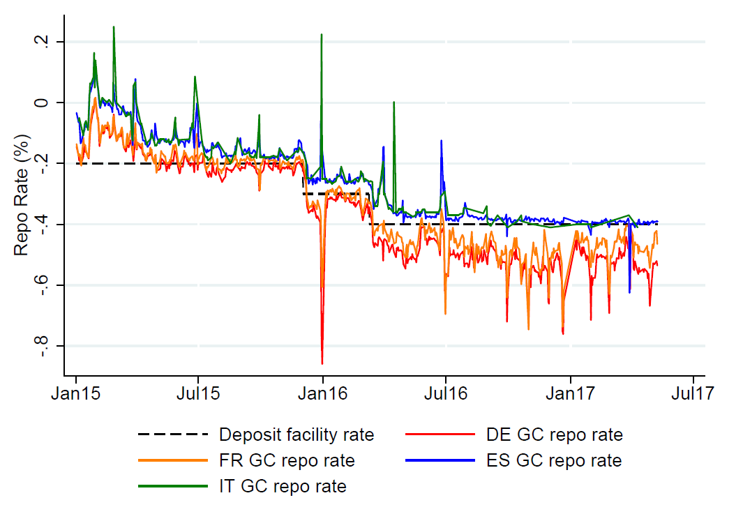
Source: IMF
(b) Spread GC repo rates and DFR against excess liquidity
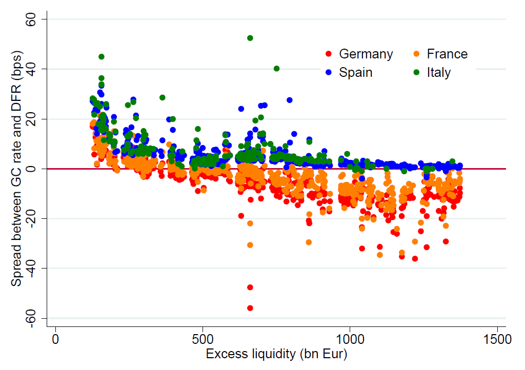
Source: IMF
As can be seen in the first figure (a), repo rates diverged more strongly and volatility overall increased after 2016. The significant spikes are due to end of year and end of quarter balancing. The differences in repo rates suggested by different jurisdictions is further represented in the elasticity to excess liquidity (figure b) where on the one hand the spread of Italian and Spanish repo rates and DFR is floored and rather inelastic with increasing excess liquidity, and on the other hand the spread of German and French repo rates and DFR is associated -1 bps with each extra €1bn of excess liquidity. Yet, in general, rates and excess liquidity seem non-linearly correlated.
The second effect, which we will only mention for the sake of completeness, is the result of portfolio rebalancing as one of the main transmission channels of asset purchase programs. Intuitively, in inefficient financial markets, those market participants that need or prefer scarce securities will be willing to bid higher to obtain them, thereby causing their prices to rise and yields to fall. Although these market participants under pressure of obtaining scarce securities will conduct purchases in the secondary cash market, while any movements in prices there will most likely affect conditions in the repo market. This relationship can be thought of simply when considering short-selling. When bonds’ prices increase as a consequence of special needs of some market participants, it will also get more difficult to borrow these specific bonds via reverse repos, thus, it can be expected that ceteris paribus, also the prices in the repo market will be inflated.
Simply put, since plenty of assets are subjected to the cash and repo market, movements in one market may influence the other.


1 Comment
D · 20 April 2021 at 13:46
Is the diagram of the repo transaction correct? The cash is sent in both examples to bank B and bank A receives the security twice? Perhaps I’ve misunderstood.