Pumping Alpha: Trading the Commodity–Currency Loop for Export Heavy Countries

Introduction

Commodity-exporting currencies are structurally linked to the prices of their primary exports through the terms-of-trade channel. While this relationship holds in the long run, short-term dislocations frequently emerge due to monetary policy shifts, capital flows, and risk sentiment. This article develops a systematic cross-asset mean-reversion strategy that exploits these temporary deviations using dynamic hedge ratios estimated via a Kalman filter. The result is a market-neutral Commodity Terms of Trade (CToT) framework designed to capture relative-value opportunities rather than directional macro bets.

The link between currencies and commodities

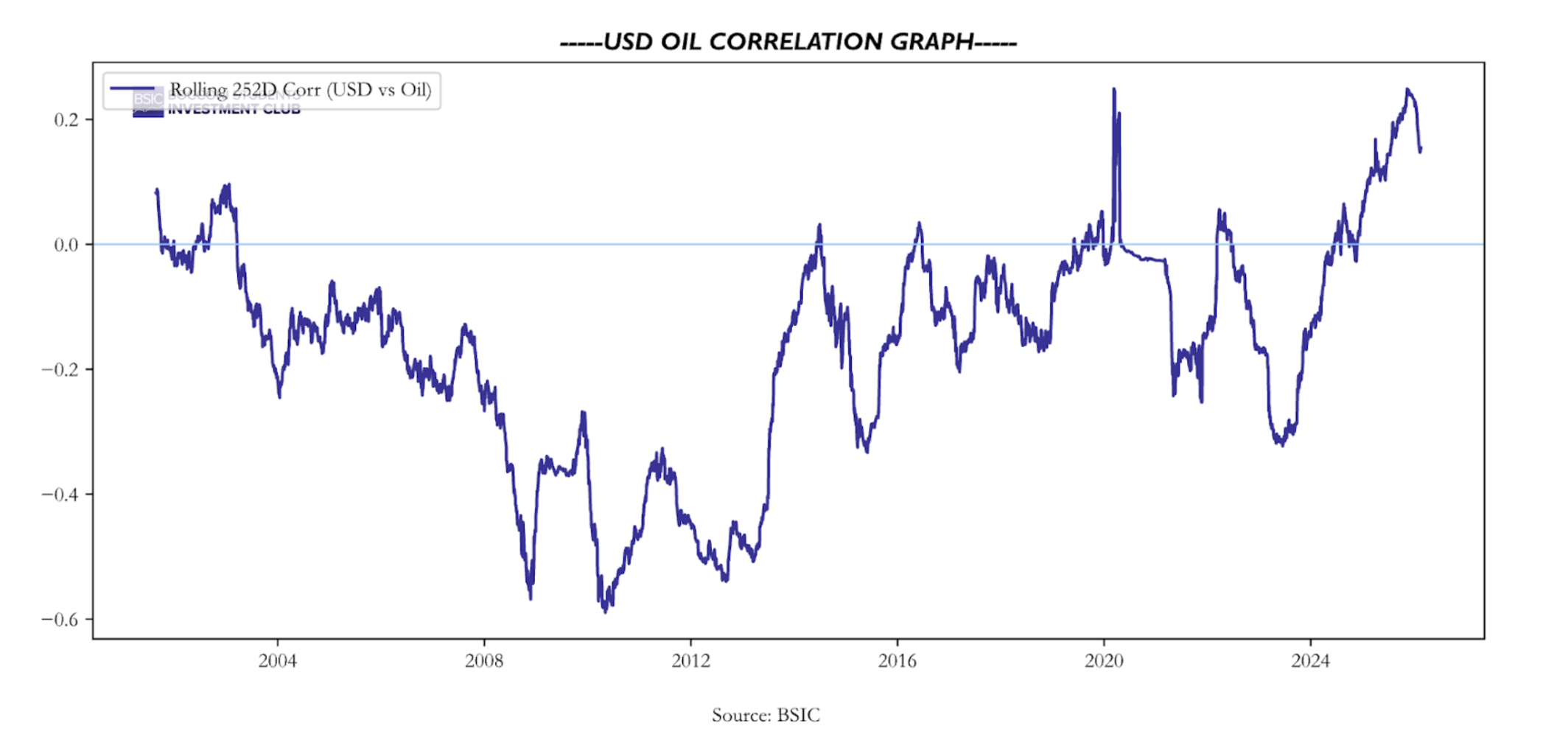
One of the most fundamental features of oil is its inverse relationship to the US dollar. The link is not trivial, rather multifaceted, but can in a general way be explained through supply and demand. Oil demand growth has been driven largely by nations outside of the United States. Because oil is priced globally in dollars, a rising USD makes the commodity more expensive in local currency terms for these international consumers. This increase in domestic cost stifles consumption, reducing overall global demand and pushing oil prices lower. A stronger Dollar also tends to boost global oil supply, particularly from producing nations with floating exchange rates. Although this is a more complicated driver, it occurs both because of improved margins and improved exports.

The relationship is one of the most studied economic relationships that still bothers traders when its dominant drivers suddenly change. The dominant factors shift frequently, leading to drastic changes in the cross-asset correlation, which also complexifies statistical modelling by making it highly sensitive to sample selection. Although the causation is either unclear or regime-changing, there is no doubt of a long-term relationship between Oil and the USD. One may initially think this relationship can come to be exploited, although to do this you must be able to find a way to eliminate less predictable factors, e.g., its impact on monetary policy, and achieve a model with stable residuals, much easier said than done. The goal of statistically debunking this relationship has been in the interest of economists, traders, and even national security since the 70s. Many attempts have also been made to establish an aggregate direction of causality. However, given so many commingled channels acting at once, disentangling causality in any robust way using statistical methods is practically impossible. While some macroeconomic changes push towards long-term equilibrium, they are still extremely slow and in the short run their combined impact is indistinguishable from non-tradable noise.

A better strategy is to narrow down the focus to a specific pair involving a commodity currency to create a more reliable statistical link. Currencies and commodities are known to have a reciprocal link where the value of a nation’s currency is heavily influenced by the global price of the primary raw materials it exports. This dynamic is what defines commodity currencies, where the exchange rate tends to track the rise and fall of specific resource markets. The dynamic primarily operates via commodity price fluctuations affecting the value of the nation’s exports relative to its imports, leading to higher revenues which in turn lead to higher demand for the local currency. Moreover, commodity-exporting countries face specific economic risks, leading their central banks to maintain higher rates to manage inflation and attract capital. In turn, this also attracts investors to perform carry trades, borrowing in low-yield environments and investing in these higher-yielding countries.

In addition to the specific relationship between the US Dollar and crude oil, our strategy adopts a broader global scope by identifying cross-asset pairs where a nation’s currency is fundamentally tied to its primary export. This expanded approach relies on the “reciprocal link” found in commodity currencies, where the exchange rate tracks the rise and fall of specific resource markets that dominate a country’s trade balance.

The commodity must account for a high percentage of the nation’s total exports, ensuring that price fluctuations lead to significant changes in revenue. We also prioritize countries where central banks maintain higher interest rates to manage inflation or attract capital and lastly look at dynamic rolling ADF tests to confirm that the residuals are stationary and mean-reverting when using a dynamic beta.

Kalman filtering

Accounting for monetary policy changes within the nations, one can expect mean-reverting behaviour between the assets, and the technical implementation of this convergence strategy is straightforward. We define the cross-asset spread as:

$\displaystyle S = CADUSD - \beta \cdot WTI$

The most challenging part of constructing a trade strategy revolving around the relationship between the assets is defining β, which is “more of an art than a science”. Trivially, a stationary beta over our defined time period is a recipe for model failure, as the sensitivity of a currency to its underlying commodity can change drastically depending on the global economic environment. A more sophisticated approach is using a rolling beta with a narrower window to allow the model to adapt to regime changes. However, rolling windows suffer from a significant lag in responding to market shifts and have a high sensitivity to the window size.

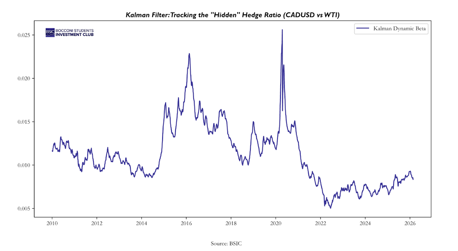
Our approach is to use a Kalman filter to allow for a dynamic beta that minimizes the drawdowns compared to those of a rolling window. A Kalman Filter is an iterative mathematical algorithm used to estimate the “true” state of a system that cannot be measured directly, especially when the available data is noisy or uncertain. In relation to our later-defined strategy, it constantly recalibrates the relationship between oil and currencies, distinguishing between temporary market noise and a fundamental shift in the hedge ratio.

The core advantage of the Kalman Filter in this strategy is its ability to maintain a smooth, yet responsive state prediction during market regime shifts.

State Prediction $\displaystyle x_p = A x_2$

Covariance Prediction $\displaystyle P_p = A P_2 A^{T}$

The model assumes that today’s beta is fundamentally linked to yesterday’s. This creates a much smoother transition compared to a rolling OLS. The smoothness of the regime shift is controlled by the Kalman Gain, which acts as a filter for noise. Because the Kalman Filter provides a more accurate and fluid estimate of the hedge ratio x₃, the resulting cross-asset spread S remains statistically stationary.

Mean reversion

Before trying to find statistical evidence of a mean-reverting strategy, one may delve into the macroeconomic relationship between the currency pair and the commodity. Currency pairs and their corresponding commodities rest on the concept of re-equilibrium. The currency of an exporting country rich in resources should reflect the value of its primary resource, and when it drifts apart, economic factors tend to pull them back together. Increased commodity prices create a positive supply shock to the nation’s terms of trade, as higher commodity prices mean more dollars flow into the producing country, and when the dollar is exchanged for the local currency, the cross-asset pair moves more in parallel. Further, central banks in commodity-heavy nations often react to commodity price swings to maintain economic stability, which reinforces the mean-reverting nature of the spread.

The residuals εᵢ are modeled as mean-reverting Ornstein-Uhlenbeck (O-U) processes:

$\displaystyle dX_i(t) = \kappa_i \big(m_i - X_i(t)\big)\,dt + \sigma_i\, dW_i(t)$

where $\kappa_i > 0$ is the speed of mean reversion, $m_i$ is the long-run equilibrium level, $\sigma_i$ is the volatility of the residual, and $dW_i(t)$ is a standard Brownian motion. This stochastic model implies that deviations $X_i(t)$ (the residuals) tend to revert toward $m_i$ over time, rather than drifting indefinitely.

In this setting, the residual tends to fluctuate around $m_i$ with a stationary variance given by:

$\displaystyle s_i = \frac{X_i(t) - m_i}{\sigma_{eq,i}}$

The s-score standardizes each residual by its equilibrium variance to measure how far it is from equilibrium in units of standard deviations:

$\displaystyle s_i = \frac{X_i(t) - m_i}{\sigma_{eq,i}}$

However, Avellaneda & Lee (2008) show that the mean term is 0, further supporting the assumption behind the mean-reversion nature of residuals. Then, the s-score can be approximated to:

$\displaystyle s_i \approx -\frac{X_i(t)}{\sigma_{eq,i}}$

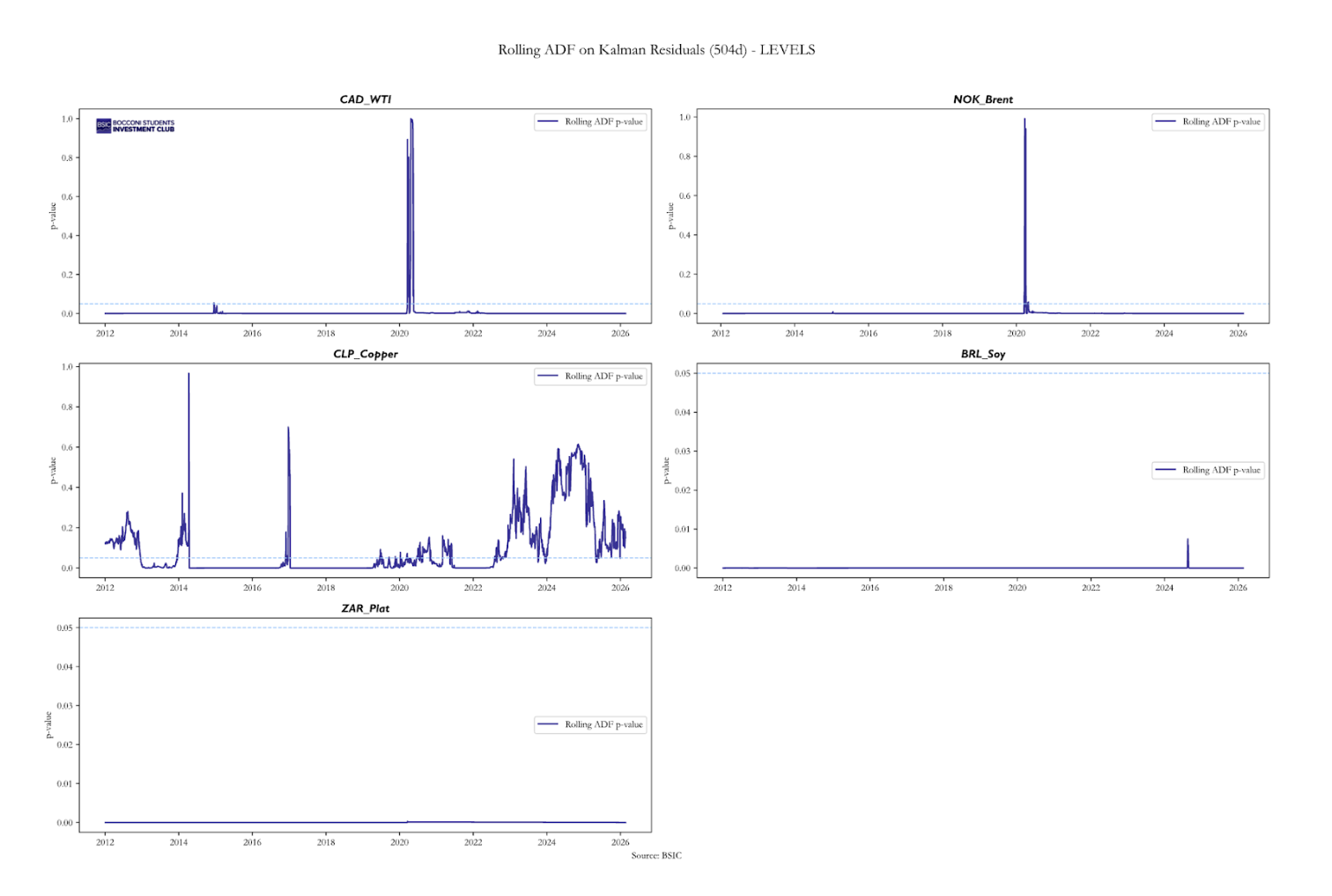
In our universe, the dynamic rolling ADF (Augmented Dickey-Fuller) test is applied to the residuals of the regression between the FX rate and the commodity price using the dynamic beta. Rejection of the unit-root null in these residuals provides evidence that the series are cointegrated over the given window. Cointegration is a statistical property that describes two or more non-stationary variables that move together over the long term such that a linear combination of them is stationary. When two assets are cointegrated, it is not the individual series that must be stationary, but rather the residual from the regression of one on the other. Beyond simple correlation, which only measures whether two variables move together, cointegration tests whether a stable long-run equilibrium relationship exists between them.

The limitations of static cointegration models are addressed by implementing a Kalman Filter to estimate a time-varying hedge ratio. While traditional Engle-Granger methods rely on a fixed beta that can break down during market shocks, our approach utilizes a state-space model where the beta is treated as a dynamic state that evolves alongside the market. By applying a dynamic rolling ADF test to the residuals generated by this Kalman Filter, we can statistically confirm that the resulting spread remains dynamically stationary even as the underlying relationship shifts.

Below we see the rolling dynamic ADF tests with p-values for the different FX-commodity pairs we chose to explore, where evidence of mean reversion is certainly strong besides some regimes. An extension of the trading strategy to be presented could be to add a p-value gate and trade only when evidence of dynamic cointegration with the Kalman beta is present.

It’s clear that in some volatile periods with differing regimes, cointegration can break and so can mean reversion, as we see a spike in p-values in 2022. However, on average we can determine that for most of the time the residuals of the spread are stationary and the relationships are mean-reverting with dynamic cointegration.

Trading Strategy

Each exporter currency embeds, in equilibrium, the wealth effect and trade-balance impact of its primary export commodity. Formally, we posit that for exporter currency.

The core economic premise is that, over the long run, exporter currencies embed a terms-of-trade/wealth effect (Commodity ↑ → exporters earn more USD → they convert USD to local currency → local currency appreciates, and vice versa) from the commodity they export. In the short run, FX can be driven by rates, risk sentiment, domestic shocks, or liquidity, causing deviations from this link. The strategy attempts to profit from the mean reversion of that deviation.

The implementation is fully systematic:

Estimate a hedge ratio (β) between FX and commodity on price levels with Kalman Filtering.
Construct a residual/spread (mispricing) using β.
Normalize it into a z-score using a moving window.
Enter positions when the z-score is extreme (We chose 2), exit when it reverts.
Risk manage via vol targeting, β-volatility throttling, z-stop, and a portfolio drawdown throttle.

We define the theoretical cross currency spread as $\displaystyle S = FX - \beta \cdot Commodity$

Commodity and estimate the dynamic equation using a state-space (Kalman filter) regression on price levels. The strategy can also be performed with a rolling OLS, but Kalman Filter regression offers a smoother beta value and provides a cleaner signal to trade with because of its state/regime-changing properties, which particularly apply well to commodity markets. While Rolling OLS assumes β is constant inside a window and then jumps when the window rolls, the Kalman Filter assumes β evolves gradually through time. The Kalman Filter treats β as a hidden state that moves slowly and continuously.

$\displaystyle FX_t = \alpha_t + \beta_t \cdot Commodity_t + \varepsilon_t$

$\displaystyle S_t = FX_t - (\beta_t \cdot Commodity_t + \alpha_t)$

With state transition $\displaystyle \beta_t = \beta_{t-1} + \eta_t$ assumed to be a random walk.

$β_t$ evolves gradually over time. Transition covariance controls flexibility. & The filter updates using only past information.

Because the hedge ratio $β_t$ evolves over time, the commodity leg must be rebalanced daily to maintain a neutralized exposure. At each time step, target holdings are updated according to the newly estimated $β_t$ , and the difference between current and target commodity exposure is traded. This ensures that the strategy remains dynamically hedged and prevents artificial PnL arising from parameter drift.

Trading Signal

We standardize deviations using rolling statistics $\displaystyle z_t = \frac{S_t - MA_{20}(S_t)}{SD_{20}(S_t)}$

$MA_{20}(S_t)$ is 20 day moving average & $SD_{20}(S_t)$ is 20 day standard deviation

Trading Rules:

$\displaystyle \pi(S_t)=\begin{cases}-1 & \text{if } z_t>2 \\ 0 & \text{if } -2\le z_t \le 2 \\ 1 & \text{if } z_t<-2 \end{cases}$

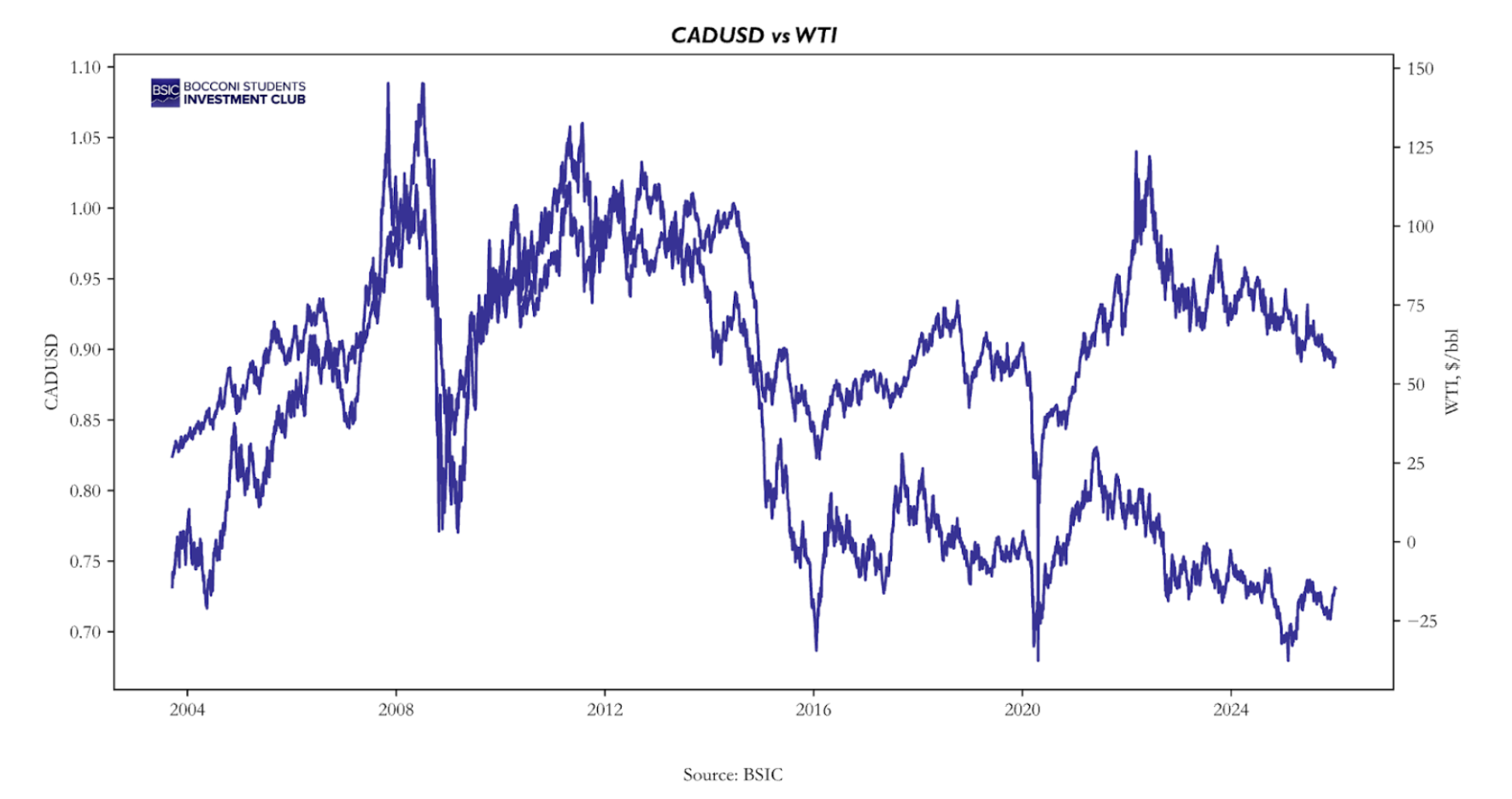
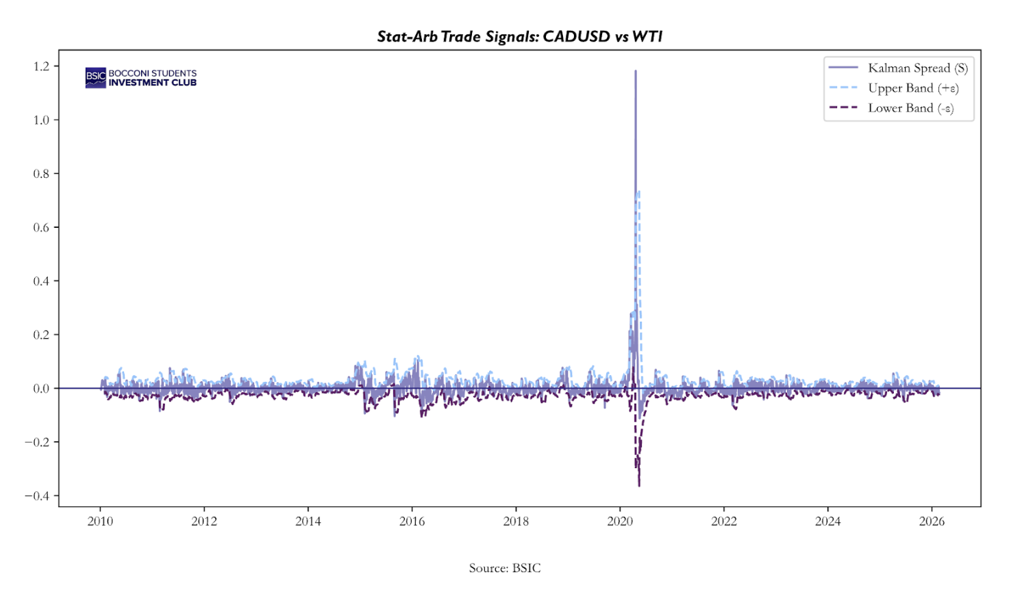
Here is an example of the signals from the CAD–WTI relationship. We see that the majority of the time the relationship remains within the bands, with some larger deviations.

Risk Management

Z-score stop:

We include a z-score stop in case deviation becomes extreme where regimes might be changing or vol is too high where we don’t trade if $|z_t| > 4$

Beta filter:

When β exhibits unusually high instability (rolling 60-day std above threshold), exposure is halved to reflect structural regime uncertainty.
Define $\beta_{vol} = \text{std}(\beta_t, 60d)$
If $\beta_{vol} > 4 \times \text{median}(\beta_{vol})$ then we reduce exposure by 50%.

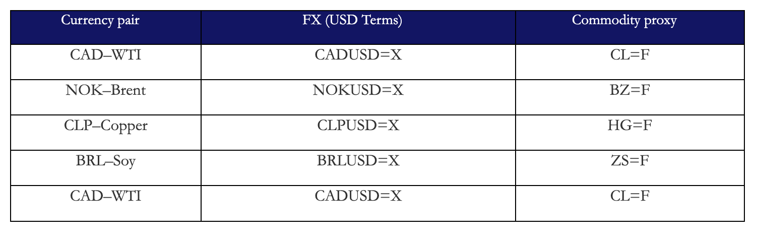
Data & Universe

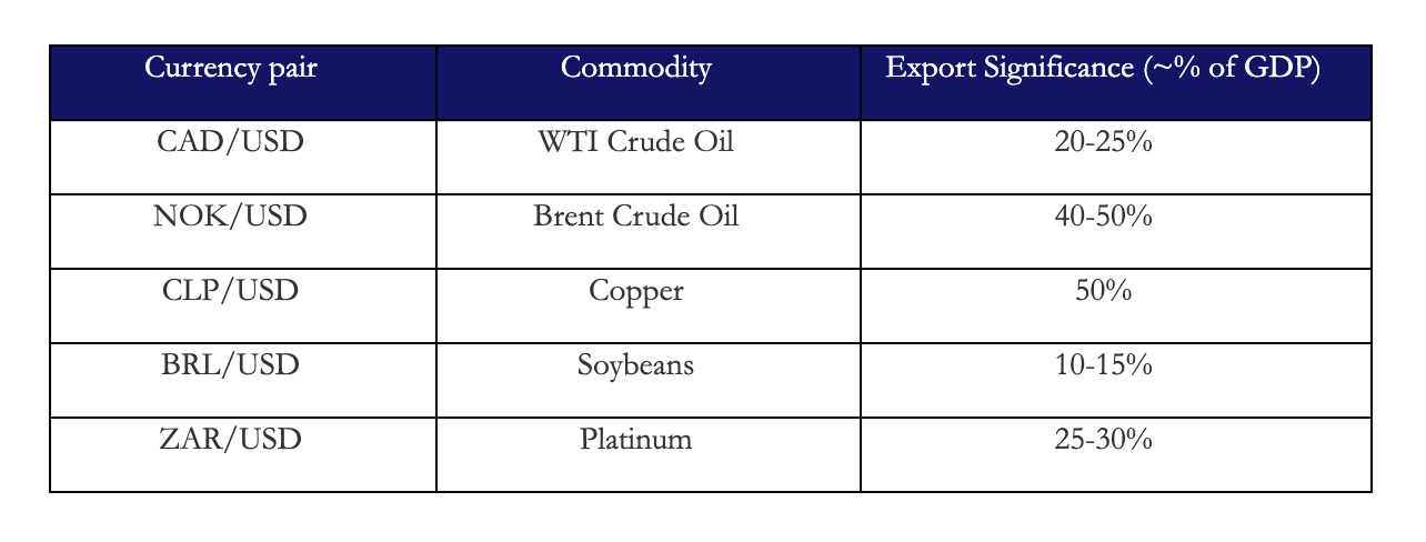
The exporter–commodity pairs were selected based on the strength, persistence, and macroeconomic relevance of the terms-of-trade channel in each economy. The core requirement is that the commodity represents a structurally significant share of national export revenues, fiscal receipts, and current account dynamics. In such settings, commodity price fluctuations have first-order effects on national income expectations, trade balances, sovereign risk premia, and ultimately currency valuation.

Portfolio construction

Combining a number of these pairs we can construct a Commodity Terms of Trade (CToT) portfolio. Benefits: Geographic diversification, Commodity diversification, less idiosyncratic risk & Smoother performance

We established the basket of 5 pairs with risk weighted total of 1/5 each. Where at each time t we had:

$\displaystyle FX_{target} = scaled_{pos}$

latex]\displaystyle Commodity_{target} = -\,scaled_{pos} \cdot \beta_t[/latex]

Long Spread = Long FX & Short Commodity (Beta scaled)

Short Spread = Short FX & Long Commodity (Beta scaled)

To risk weigh the portfolio we begun by setting a total portfolio volatility target which we choose to be 30% since we have low vol for each pair weightings will come out to be roughly 10% overall portfolio vol.

Each pair targets a fraction (0.2) of 30% annual portfolio volatility:

$\displaystyle \sigma_{daily\,target} = \frac{\sigma_{ann\,vol} \cdot risk\ weight}{\sqrt{252}}$

$\displaystyle Scale = \min\left(\frac{\sigma_{Target}}{\sigma_{Realized}}\right)$

In this way we can prevent: Single pair domination (especially since the risk / vol of each pair will differ significantly), idiosyncratic Commodity shock blow-ups & EM FX volatility concentration.

Transaction costs

We assume 5 bps on commodity hedge adjustments and explicitly deducted from PnL.

Results

Regarding trading frequency, the mean holding time is roughly 2.5 days. This means this is not a slow macro convergence strategy. It is closer to short-horizon statistical reversion. However, per pair we only enter trades roughly 12 times per year. This means we are not seeing long macro convergence or multi-week equilibrium reversion, but rather short-horizon reversion occurring infrequently. This also indicates that if we loosened our entry criterion, we could see more trades and perhaps a larger trade sample size could result in lower volatility.

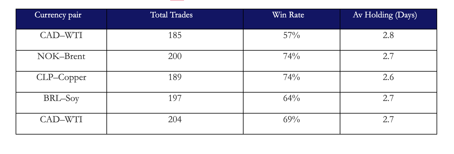
As we see even though we don’t enter in many total trades we have very significant win rates which translate to performance.

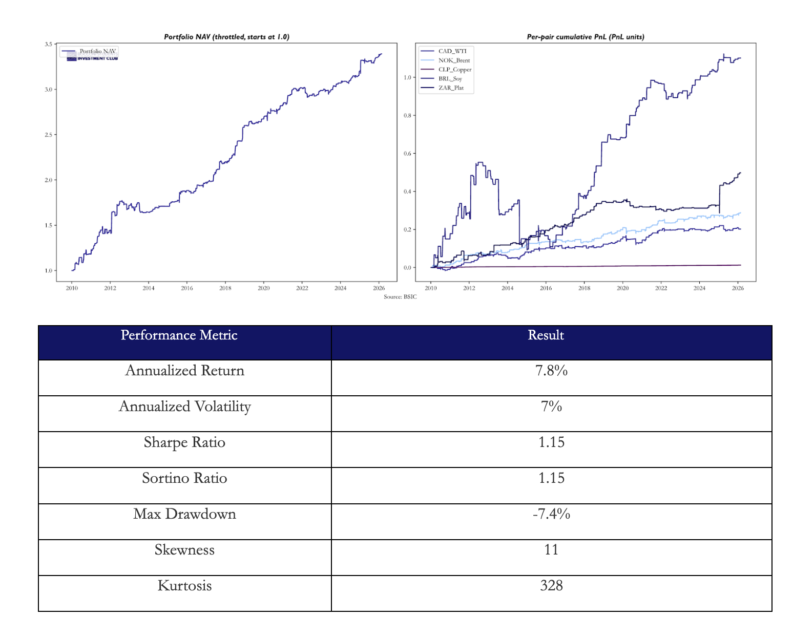So far, it delivers strong absolute returns for a market-neutral relative-value strategy, if performance is achieved without meaningful exposure to standard equity or macro risk factors.

The Sharpe ratio indicates solid risk-adjusted performance and suggests returns are efficiently generated relative to volatility.

What stands out most is the skewness (11). Unusually high positive skew suggests occasional large upside moves. This warrants verification to rule out distributional distortion. Kurtosis (328) is extremely elevated and indicates very fat tails or outliers. This metric requires further robustness checks to confirm stability.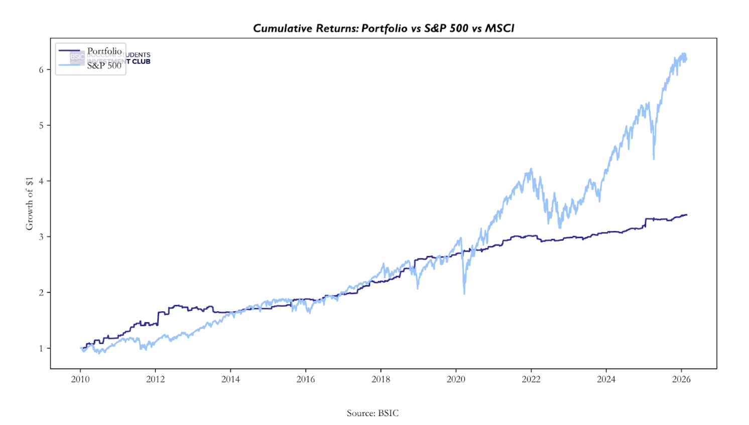Relative to the S&P 500 (our chosen benchmark of the universe’s market), it is clear that our strategy tended to underperform in terms of annualized returns but outperform in terms of annualized volatility (7% vs 17%) and Sharpe ratio (1.1 vs 0.7).

The question naturally becomes: is this just beta, or is it indeed the stationarity of residuals that dominated the return profile?

Factor Analysis

To assess whether the strategy generates genuine abnormal returns (alpha) or merely harvests systematic risk premia, we regress monthly excess strategy returns on standard risk factors taken from the Fama-French database.

We first estimate the following specification:

$\displaystyle R^{excess}_{strategy,t} = \alpha + \beta_{MKT} MKT_t + \beta_{SMB} SMB_t + \beta_{HML} HML_t + \beta_{MOM} MOM_t + \varepsilon_t$

where:

MKTis the market excess return, SMBis the size factor, HMLis the value factor

The regression yields: R² = 0.01, All factor loadings statistically insignificant Intercept (α) = 0.0061 monthly, statistically significant (p < 0.01).

Only 1.7% of return variation is explained by common equity risk factors. The lack of statistically significant exposures to MKT, SMB, or HML suggests the strategy is not simply a disguised equity or factor rotation strategy. The positive and statistically significant intercept indicates that returns remain unexplained by standard risk premia.

Importantly, we maintain a No-Alpha prior. While the intercept is consistent with abnormal returns, further robustness testing is required before concluding the presence of structural inefficiency.

To further test whether the strategy is implicitly exposed to broad macro drivers, we estimate:

$\displaystyle R^{excess}_{strategy,t} = \alpha + \beta_{SPX} SPX_t + \beta_{DXY} DXY_t + \beta_{COM} COM_t + \beta_{dTNX} \Delta TNX_t + \varepsilon_t$

using Newey-West (HAC) robust standard errors.

Regression results: R² = 0.046 All macro betas statistically insignificant expect intercept (α) = 0.0064 monthly (0.64% monthly ~5% yearly), statistically significant (p < 0.01).

Only 4.6% of monthly return variation is explained by broad macro factors. The absence of significant exposure to SPX (equity beta), DXY (USD strength), COM (commodity beta), or changes in rates confirms that the strategy does not behave as a directional macro trade.

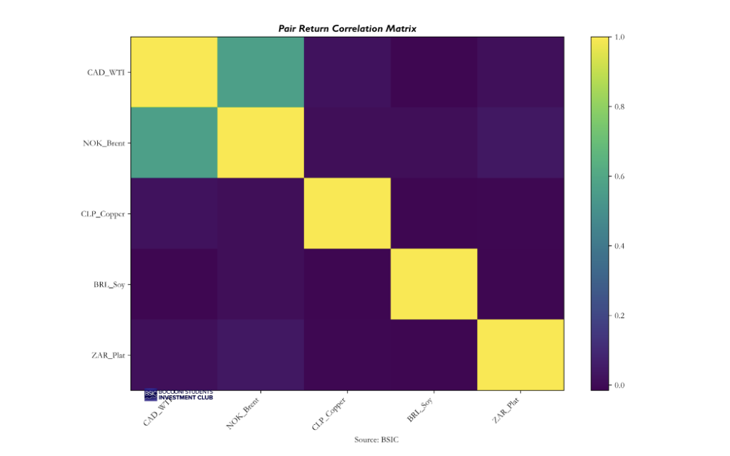
Furthermore, running correlation analysis, we see the pair returns are not highly correlated with each other or any macro variable except for CAD–WTI & NOK–Brent, which have a correlation of 0.567, the highest of all.

Regarding macro variables, our portfolio had correlations for monthly returns of 0.005 with the S&P, 0.006 with WTI, and 0.005 with DXY, providing further evidence of robustness as an independent source of returns.

Risks

To maintain a realistic perspective of the model, we must account for primary risks. The most critical risk to this strategy is a breakdown in the fundamental reciprocal link between a currency and its commodity. Usually, an oil-producing nation’s currency rises when global oil prices spike. However, if a major exporter faces domestic instability, its production may fall while global oil prices spike due to the supply shortage. Investors may have the incentive to pull out of the unstable currency, creating a “double whammy” loss.

Moreover, our strategy assumes that the wealth effect from commodity exports will naturally translate into currency demand, but if the Federal Reserve enters an aggressive tightening cycle while a commodity-producing nation keeps rates low to stimulate a weak domestic economy, the USD may appreciate despite rising commodity prices. This may cause our spread to drift so far that it fails the Rolling ADF stationarity test, rendering the mean-reversion signal invalid.

Regime Analysis

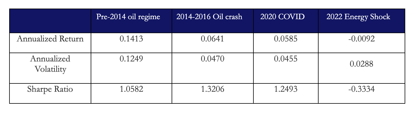As we can clearly see, our model holds up during geopolitically uncertain regimes, with deviating drawdowns during the 2022 energy shock. A viable argument for why the strategy succeeded pre-2020 (inclusive) is that the fundamental drivers of commodity currencies stayed intact. During the 2014 crash and the 2020 pandemic, the “wealth effect” continued to function. Even during the extreme volatility of 2020, the Kalman Filter was able to smoothly update the beta. This kept the residuals stationary, allowing the strategy to capture profits as the spread reverted to its mean.

The 2022 Energy Shock represents a total breakdown of the cointegrating relationship, evidenced by the negative Sharpe Ratio of -0.3334. As discussed in the risks segment, the failure might be an indicator of the “double whammy” risk. While energy prices spiked in 2022, many producer currencies did not appreciate at the expected rate due to domestic instability and massive capital flight. Lastly, the US Federal Reserve raised interest rates more aggressively than many commodity-producing nations. This strengthened the USD against currencies like the CAD or NOK even as oil prices rose.

Conclusion & Improvements

While the strategy is economically intuitive: exporter currencies should reflect the value of their primary commodity, the existence of apparent alpha must be approached with caution. The edge does not arise from forecasting commodity direction, but from exploiting temporary dislocations between structurally linked markets. Such deviations can persist due to capital flows, monetary regime shifts, liquidity frictions, and risk-premium adjustments, which are not instantaneously arbitraged.

Nevertheless, we maintain a strict “No-Alpha” prior: intuitive logic and backtest performance alone are insufficient proof of inefficiency. The strategy’s viability ultimately depends on robustness to transaction costs, regime shifts, parameter sensitivity, and out-of-sample testing. If the signal survives these stresses, it likely represents a structurally persistent cross-asset relative-value opportunity rather than a backtest artifact.

References

Bouchouev, Ilia, “Virtual Barrels, Quantitative Trading in the Oil Market”, 2023

Published by BSIC on 22 February 202622 February 2026

0 Comments

Leave a Reply Cancel reply

Market Recap 22/02/2026

Rates Up, Yen Down: Japan’s Currency Paradox and What Comes Next

A Friendly Introduction to Money Markets