Quick recap
In the last newsletter we published an article providing the theoretical foundations of Dispersion Trading (in case you missed it: https://bsic.it/lost-dispersion-trading/). As promised to our readers, here is a follow up with some real market applications. However, you still need to wait for the chapter III in the next newsletter to see the final results.
Data
The empirical investigation focuses on the dispersion trading strategy using S&P 100 index options and individual options on all the stocks included in the index. The S&P 100 Index is a subset of the well-known S&P 500 containing the shares of the 100 biggest US companies. Therefore, in order to set up a dispersion trade, we need data on the options on the S&P 100 Index as well as those on the components – remember that our objective is to obtain opposite exposures on the Index and Components options. Specifically, we need historical data on Closing Prices and Shares Outstanding of the underlying stocks and Closing Bid and Ask quotes, Implied Volatilities, Delta and Vega sensitivities for all options available.
We downloaded all these data from Wharton’s Optionmetrics, one of the leading database as far as historical options data are concerned.
Our analysis covers the period May 17, 2003 through April 15, 2016. Due to the unavailability of some Index Components’ data for the whole period considered, we end up having 71 components on top of the Index itself.
Avoiding overshooting: smartly selection of the components
Whenever fees are incurred to make a transaction, being parsimonious could payoff. This is exactly why we do not use all the individual components of the Index to perform our trade. In other words, supposing we enter a long dispersion trade, we would short the option on the Index and at the same time we would acquire a long position on options on a certain number of pre-selected components (<100 !).
By selecting a subset of the component stock options to execute the dispersion trades, we are actually reducing the transaction costs involved in the strategy, which consequently might increase the return after transaction costs.
In the selections of the Index components, we follow a procedure set out in “Hedging Basket Options by Using a Subset of Underlying Assets” [Su (2005)]. This method employs Principal Components Analysis, which through a clever re-arrangement of the data, allows to reduce the dimensionality of the data, minimizing the loss of information. After the PCA analysis is performed on the underlying assets, we end up having a factor ranking. Factors are ranked in a descending order of the percentage of the total data variance explained by them.
Then, we choose the first factors that, cumulatively, explain 90% of the variance. In this way, we reduce the dimensions in our data giving up only 10% of the variance (which could be thought of as the information contained in the data).
We can now choose the components to pick in this way: select the n index components whose returns had had in the period considered the highest cumulative correlation squared with the Principal Components selected in the previous step. In our case, n is a-priori set at 15. Why 15? Because we found qualitatively that adding more components would slightly improve the cumulative correlation squared at the margin (i.e. we would not be that much better off with 16 components).
Finally, we calculate the weight of the chosen components in the index by regressing the index returns against the components return.
After the subset of stocks is selected, we implement the dispersion strategy by buying (selling) the index options and selling (buying) individual options on these 15 stocks.
Enter and exit timing with the dispersion indicator
The dispersion indicator is the same as the one we mentioned in the previous article:
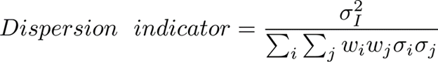
It is the index IV, divided by the volatility of a hypothetical portfolio of index constituents with perfectly positive pair-wise correlations. One key point is that we are taking the constant 1-month implied volatility from the index and the constituents options. The indicator shows a mean-reverting behavior as in chart 1.
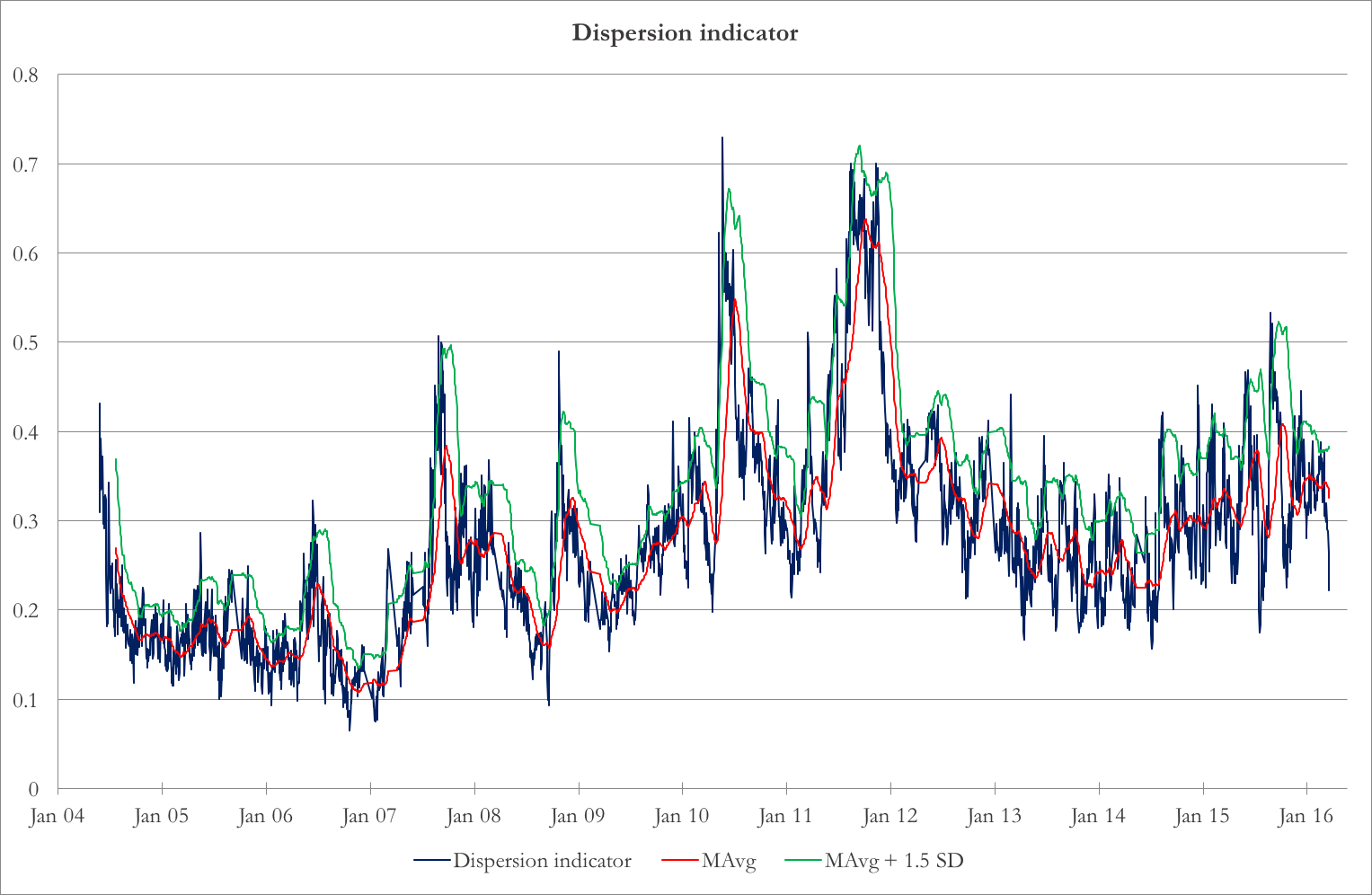
Chart 1: Dispersion indicator, together with 40-day moving average and 40-day moving average + 1.5 rolling standard deviation
Source: BSIC, Wharton Optionmetrics
We use Bollinger Bands for entry and exit timing. We find the 40-day moving average and standard deviation of the dispersion indicator. Then, we calculate the Z-score of the latest reading. Whenever this Z-score goes beyond 1.5, we enter the trade – short index volatility and long constituent volatility. We square off the trade when the Z-score hits 0.5 or at options expiry, whichever happens before.
Replicating quasi-variance swaps
The last ingredient to our arbitrage potion is to buy and sell options on the index and the components in a way that, as already written in the chapter I of this trilogy, would lead to a low delta (so that we don’t need to frequently delta hedge) and to a position which is as sensitive as possible in terms of vega.
Straddles or strangles would be enough to address the former issue but not to deal with the latter. That is why we decide to replicate (i.e. buy or sell) quasi-variance swaps. In particular, every time we enter in the position we sell (buy) six options on the Index and buy (sell) six options on each of the 15 components. Among the 6 options, we would have 3 calls (2 OTM and 1 ATM) and 3 puts (2 OTM and 1 ATM).
Moreover, the position would allocate 1/K^2 of weight to each option, where K is the strike of that option.
Mathematically we are discretizing a lot (as in principle we would need an infinite amount of calls and puts with a infinite dense strike grid) the following formula which is behind the replication of a variance swaps and of the CBOE VIX Index.
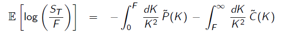
This is the cleanest way to be exposed to volatility in a model-free setting – of course our discretized position is just approximating. However, we believe it is still better than both a straightforward delta-hedged position, where we would either have imperfect hedging or high transaction costs due to continuous hedging and of straddles or strangles (with equally weighted calls and puts regardless of the strike) where we would run out of gamma and vega in a faster way.
Assigning portfolio weights
Once we have built portfolios which replicate quasi-variance swaps, we have to determine the weights of these portfolios in the overall strategy. As we are interested in changes in IV, we use the portfolios vegas as reference. We assign the weights determined by the PCA to the Vega of the index options portfolio to determine the optimal vega of the portfolios of constituents’ options. The formula is:
Required Vega for j-th component = Index Vega exposure x weight of j-th component in the index
To calculate the required number of portfolios of components’ options, we find:
Number of portfolios on j-th component = Required Vega for j-th component/Vega of j-th component portfolio
Note that in this way, we will get the number of single option as non-integers. To avoid this minor problem we scale up the number of portfolios on each component by a large number and round it off to the nearest integer.


0 Comments