Introduction
A yield curve depicts the returns of fixed income securities against their term, or time to maturity. In this article, we explain the role that the discount function and forward rates have in the creation of a yield curve and compare different methodologies to fit the yield curve, namely, bootstrapping, spline-based methods, parametric and nonparametric models. Finally, we conduct an analysis specifically on the Nelson-Siegel and Wiseman models.
Discount Function and Yield Curve
The most important function used to understand the term structure of interest rates is the discount function  , which represents the present value of $1 repayable in
  years. We expect this function to be continuously differentiable and monotonically decreasing, due to the time value of money. The function can be represented as follows:

This is the discrete version of the formula where  represents time in years and
  is the risk-free rate at time . By deriving the limit as time intervals go to 0, we obtain the formula for continuous discounting, which allows for a smoother and more precise curve:

where the first variable is the start time of the discounting and the second one is the time when the payment is received. From this continuous discount function we can derive, for instance, the spot 1Y rate  , and the spot 2Y rate
  . Hence, we can compute the forward 1Y1Y rate, another central component to the construction of a yield curve:

This comes from the no-arbitrage condition which states that must equal  . We can clearly see that the forward rate is positive, which is consistent with the discount function decreasing. It can be expressed more clearly with this notation:

This formula can also be expressed in the general form:  , which is crucial to derive the instantaneous forward rate function:

With this relationship, we can observe that when the yield curve is in its “normal” upwards sloping state, the forward rates will lie above the yield curve, and that they will lie below the yield curve when it is inverted. By integrating on both sides, we can isolate  and obtain a formula for the yield curve:

The Importance of the Yield Curve
To understand why these calculations are made, it is pivotal to comprehend the importance of the yield curve. Firstly, the yield curve serves as an indicator of the overall environment of an economy. When the yield curve is in an upwards sloping, “normal” state, it indicates the economy is expanding. On the other hand, an inverse yield curve has historically been a predecessor to a recession, as discussed in this article. We are currently witnessing a period where the yield curve is inverted, and so far, markets have responded accordingly, with 2022 being a disastrous year for equities world-wide.
Another, possibly more important and relevant use of the yield curve, is bond pricing across all possible maturities, not only the on the main liquidity points such as the 2Y, 5Y, or 10Y Treasury. This is relevant due to the fact that having the ability to accurately price a bond at any maturity lays the foundation for Relative Value strategies, one of the two main strategies implemented in rates trading. Relative Value strategies rely on the evaluation of whether a bond is trading too “rich” or too “cheap” at any given maturity, which is why constructing a yield curve is the foremost important tool in making these evaluations. When a bond is trading “rich” it means that it has a lower yield, or a higher price than bonds with similar credit risk and time to maturity. The opposite is true for when a bond is trading “cheap”.
Spline-based Methods
One of the earliest methods for fitting the term structure of interest rates was proposed by McCulloch (1971). It consists of a linear regression of the discount function which is assumed to be expressed as a linear combination of  differentiable functions
  plus a constant term
  , that is:

The present value of $1 paid back instantly is $1, that is  , which implies that
  and
and  . Recall that the price
  of a bond with constant and continuous coupon
  , principal
  and maturity
  is:
is:

combining the two equations above yields:

where  and
and  . Now, let us move to multiple dimensions and consider
  observations of bonds. To take into account errors in the bond pricing formula due to factors such as transaction costs, callability and tax exemption, we introduce an error term in the formula for the bond :

where  is the average between bid and ask, and
  is the error term. The standard error (S.E.) of is assumed to be of the form
  , where
  is the bid-ask spread. Consequently,
  for a bond becomes:

The only unknowns are the  ’s and
  , which can both be estimated through a weighted least-squares regression of the vector
  on the matrix
  , obtaining
  . We can now estimate the discount function:

and finally the yield curve:

As for the choice of , if it is too low it might not fit the discount function well, while if it is too high it will overfit outliers, compromising the smoothness of the curve. The best choice is the one that minimizes the variance of the residuals. The functions can be chosen arbitrarily, as long as they are continuously differentiable and  . Since maturities are not uniformly distributed, ideally
  provides more resolution when maturities are clustered, which in the case of Treasuries occurs in the short term. The simplest approach would be:

This choice of functions makes  a -th degree polynomial, but it does not respect the criteria on resolution. For this reason, McCulloch (1971) and McCulloch (1975) adopt quadratic and cubic splines, which are piecewise polynomial functions that interpolate a set of nodes, i.e. yields at known maturities. In particular, cubic splines are twice continuously differentiable and exhibit great flexibility when fitting the yield curve.
Later on, new methods have been developed, such as Vasicek and Fong (1982), which relies on exponential splines to replicate the exponential nature of the discount function, as well as Adams and Van Deventer (1994), which maximizes the smoothness criterion  by fitting the forward rates curve with a fourth-order spline without the cubic term.
Parametric Models
Parametric models define a specific functional form to fit the term structure. One of the earliest models was presented by Cohen, Kramer and Waugh (1966), and it consists of a multilinear regression of the yield on the days to maturity and on the squared log of days to maturity. It was later revisited by Echols and Elliot (1976) that performs a linear regression of the form:

Currently, one of the most used parametric models was proposed by Nelson and Siegel (1987). It specifies a functional form for the instantaneous forward rates, given by the solution of a second-order differential equation:

This model is consistent with the three factors of the term structure proposed by Litterman and Scheinkman (1991): level, slope, and curvature. Moreover, its formula captures some key properties of the forward rates curve, namely being monotonic, humped, and S-shaped, by modeling the following parameters:
- Level
 : long-run level of interest rates (strength of long-term component);
 - Slope
 : spread between short term and long-term interest rates (strength of short-term component);
 - Curvature
 : magnitude and direction of the hump (strength of medium-term component);
  : shape parameter, position (in time) of the hump.
The yield curve can then be derived:
![r(m)=\beta_0+(\beta_1+ \beta_2)[1-exp(-\frac{m}{\tau})]\cdot(\frac{\tau}{m})-\beta_2 exp(-\frac{m}{\tau})](https://bsic.it/wp-content/ql-cache/quicklatex.com-ed44ca1d2581e7976d8b273e479476de_l3.png "Rendered by QuickLaTeX.com")
where the estimators of , and can be calculated through Ordinary Least Squares (OLS), while the shape is the optimal one among a grid of values (grid search): this procedure is preferred to the one which estimates all parameters simultaneously through nonlinear regression. Ridge regression is usually employed to address multicollinearity, as proposed by Annaert (2012).
One of the key points of the Nelson-Siegel model is its asymptotic behavior in the long run, which reflects the fact that real yields tend to converge to a constant level at long maturities. Moreover, the model describes the typical hump that can be found in a forward rates curve. On this regard, Svensson (1995) proposes an improvement of the Nelson-Siegel model with two humps, consequently including new parameters  and
and  which represent the magnitude and the position of the second hump:

Other parametric models include Wiseman (2012):

where an OLS is performed after fixing values for  , for instance, 12 years, 5 years, 2 years, 6 months, and 1 month. Intuitively, as in Nelson Siegel, each
  affects different regions of the curve, depending on the values of the .
LMNT Kernel Estimation Method
A substantial improvement in performance compared to the McCulloch spline methods (1971, 1975) comes from the non-parametric kernel smoothing procedure developed by Linton, Mammen, Nielsen and Tanggaard (2000). To give some mathematical background needed to understand the model, we briefly discuss the definition of a Kernel Density Estimator (KDE). We define KDE for a bandwidth  as follows:
 .
.
Where our function  is called a Kernel and is defined as Lebesgue integrable function that satisfies the condition
  . Although there is a wide variety of usable Kernels, one of the preferred ones in practical uses is the Gaussian Kernel, which is also adopted in the LMNT model. We define the Gaussian Kernel as
  .
.
The LMNT model studies in depth two main estimators, the “local constant” and “local linear” methods, which locally approximate the discount function as a constant and a linear function of maturity. Once again, we define the yield curve for a maturity as:  . This approach displays a few fundamental advantages, namely that , that
  and finally that it is closer to being log-linear than linear. According to the model, we can approximate the yield curve as a linear function
  where
where  is known maturity close to . From this relationship and from the formula of the present value of a bond , our estimated present value is as follows:

Our estimation model is based on minimizing the sum of squared pricing errors: particularly, we want to find a function  and its first derivative such that with respect to the actual yield curve the following criterion is minimized:

with being our Kernel function,  as our bandwidth and
  .
.
A simpler way to obtain a result is by solving the two first order conditions that derive from the minimization problem above for our actual yield curve and its first derivative, namely:


with

Given the following framework for our model, we need to pick a few elements that are necessary to carry out the estimations of and its derivative: in this decision, we will report the methodology of Jeffrey et al. (2000). Firstly, as briefly mentioned, we will use the Gaussian Kernel for our density estimation; secondly, in order to pick the appropriate bandwidth, we observe that cash flows generated by bonds of longer maturities tend to be more sparse, thus calling for to be a function of maturity when computing the present value of the  cashflow. The paper suggests an increasing linear relationship of the form
  with
with  and
and  , allowing for greater flexibility in the front-end of the curve, where more information is available. Lastly, we pick a finite set of maturities
  to be used to compute our estimated and
  . Our set of maturities is calculated as
  and
and  .
.
Theoretically, given our first order conditions we could compute any possible , but for practical reasons we need to work with a finite set and interpolate between the calculated points. The interpolation procedure aims to minimize our original criterion obtaining an estimated pure zero-coupon bond:

Fama-Bliss Bootstrapping
One of the more classical methods to estimate the yield curve, which displays a tremendous accuracy in the front-end of the curve (but it’s fairly imprecise in estimating maturities longer than one year) is the bootstrapping procedure elaborated by Fama and Bliss (1987).
The process is of iterative nature, where starting from the relationship between the forward rate  and the discount function we then assume that the forward curve is constant between successive observed bond maturities. That is, for a time-to-maturity interval
 ![(m^{i-1}, m^i]](https://bsic.it/wp-content/ql-cache/quicklatex.com-350a9050b3429ce76f7dba6e5d571c4e_l3.png "Rendered by QuickLaTeX.com") ,
,  for the bond .
Given this assumption, our discount function takes the following form:  . We can then extract the price of the bonds, starting from the shortest maturity one
  , which is
  ; from this,
  given
given  and so on. The great advantage of the method is that all in-sample bonds will be perfectly priced and, generally speaking, the method displays a high degree of reliability for out-of-sample ones, even though this is limited to the short-term contracts (<1 year).
Analysis of Parametric Models
The dataset on which we conduct our analysis is published by the U.S. Department of the Treasury, and it comprises two years of daily treasury par yield curve rates, with maturities ranging from one month to 30 years. The par yield curve assumes that the price of the bonds that lie in the curve is equal to their face value, not their market value. On the par yield curve, the coupon rate will match yield to maturity, which is why the bond will trade at “par”. This curve is used to determine the coupon rate that a newly emitted bond, with a given maturity will pay in order to sell at par today.
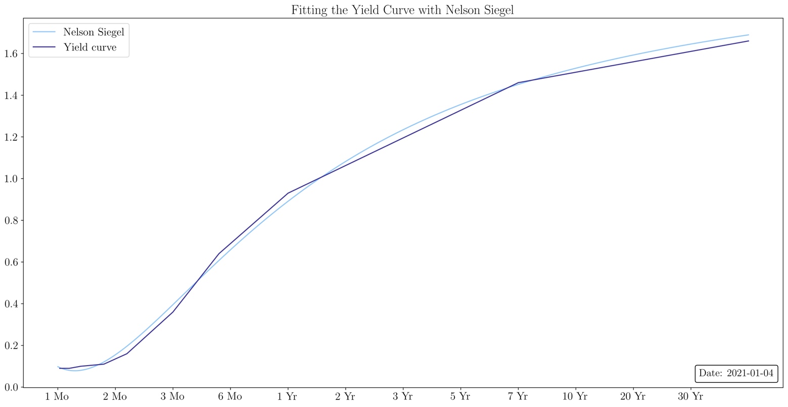
For each trading day we fit the curve with the Nelson-Siegel model, by estimating the parameters , and with OLS, and with a grid search that ranges from  to
to  and minimizes Mean Absolute Percentage Error (MAPE).
Source: U.S. Department of the Treasury, Bocconi Students Investment Club
Source: U.S. Department of the Treasury, Bocconi Students Investment Club
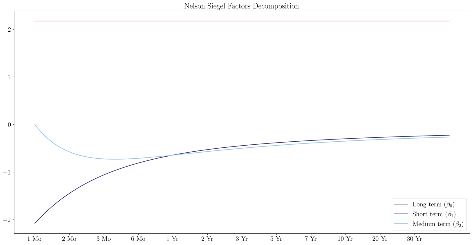
In the pictures above we observe how the Nelson-Siegel model fits the yield curve as well as the decomposition of the effects of its parameters. We can expand this analysis on the whole dataset by studying how the model’s parameters have changed over time.
Source: U.S. Department of the Treasury, Bocconi Students Investment Club
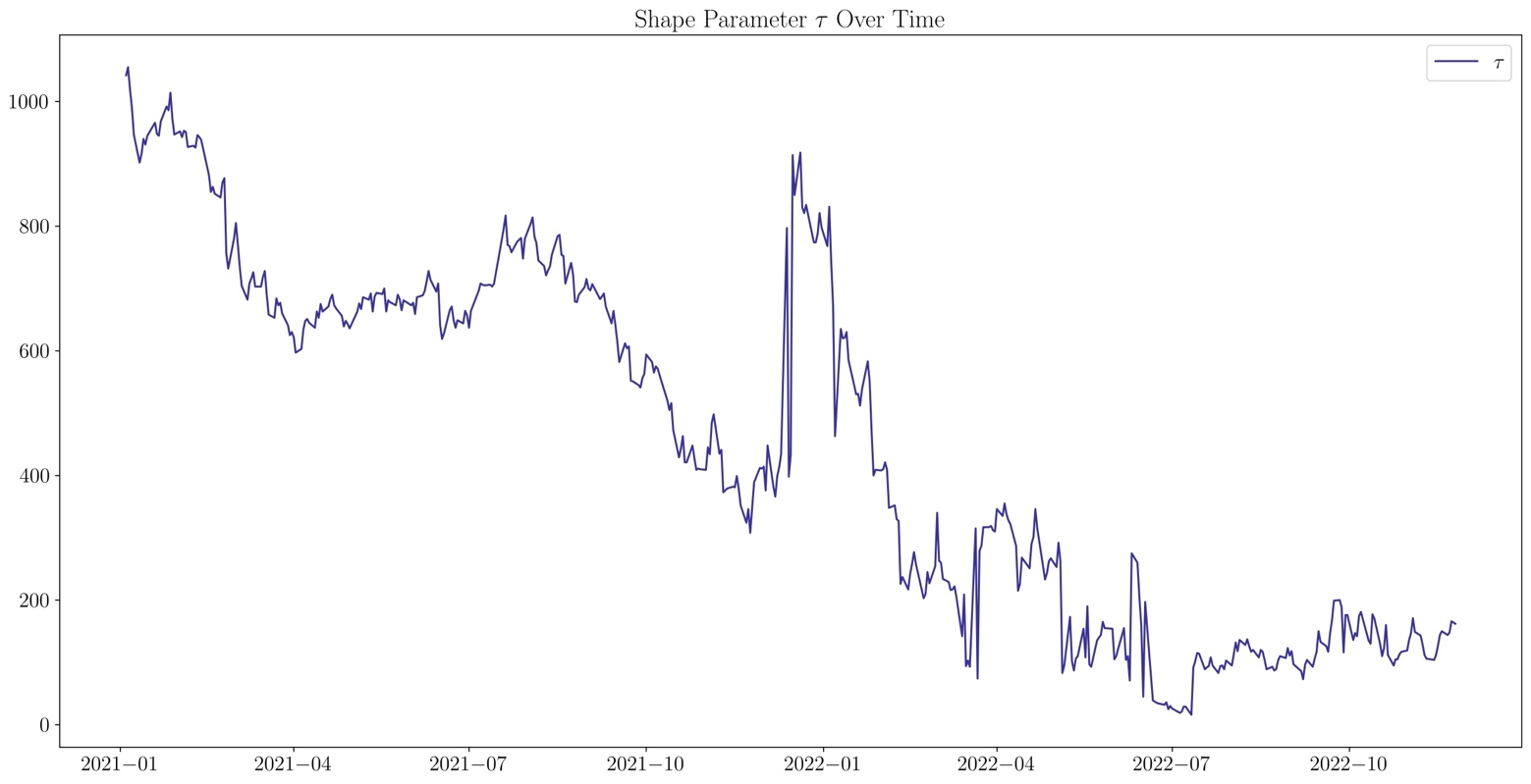
The shape parameter has decreased steadily in the last two years, expect for a spike at the end of 2021. This means that the hump of the yield curve gets nearer to the short-term maturities. It is important to note that a high value of the shape parameter may signal the absence of a hump or the presence of two humps, a case which is covered only by the Svensson model.
Source: U.S. Department of the Treasury, Bocconi Students Investment Club
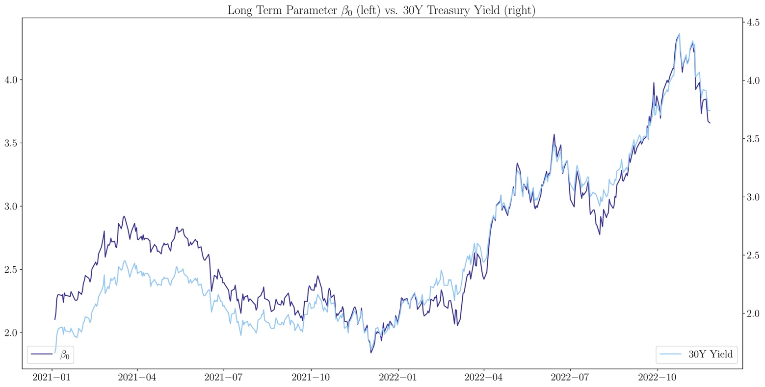
The long-term parameter essentially represents the asymptotic behavior of the yield curve, therefore it has high correlation with the 30Y Treasury Yield, with a Pearson coefficient of 0.96.
Source: U.S. Department of the Treasury, Bocconi Students Investment Club
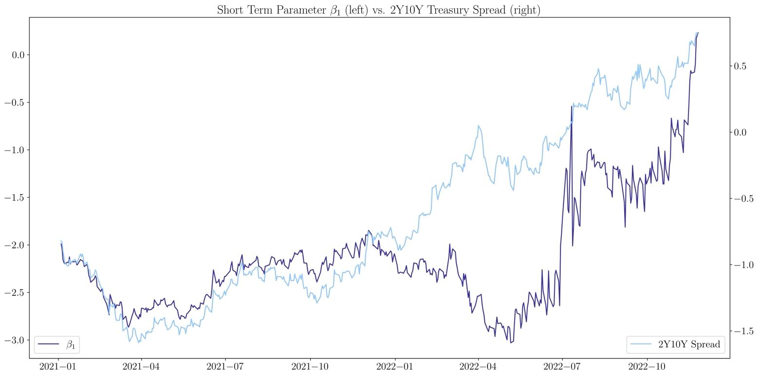
The short-term parameter depicts the slope of the curve, when it is negative the curve is in its normal increasing shape, when positive the curve is inverted. It exhibits a strong correlation (Pearson coefficient 0.7) with the 2Y10Y Treasury spread, which breaks from January 2022 to May 2022.
Source: U.S. Department of the Treasury, Bocconi Students Investment Club
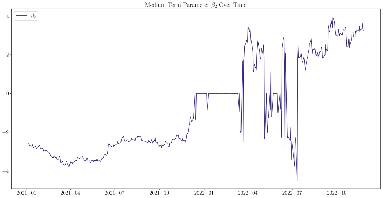
The medium-term parameter is the most difficult to interpret due to its oscillatory behavior. We observe that in the period from January 2022 to March 2022 the parameter is almost constantly set to 0, resulting in a simplified model that generates a monotonic yield curve, without curvature effect.
Source: U.S. Department of the Treasury, Bocconi Students Investment Club
Source: U.S. Department of the Treasury, Bocconi Students Investment Club
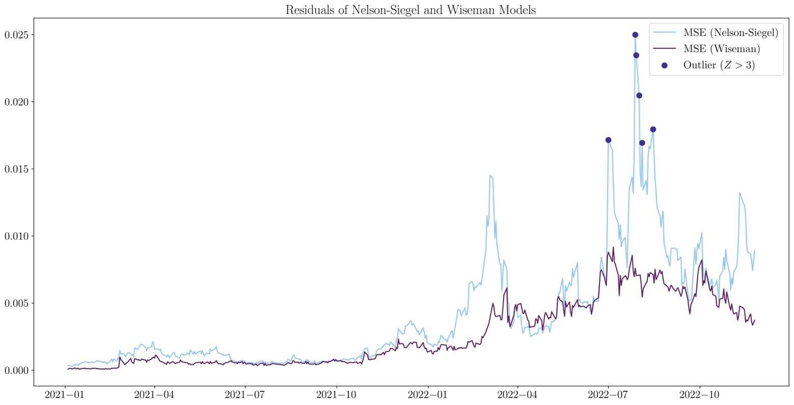
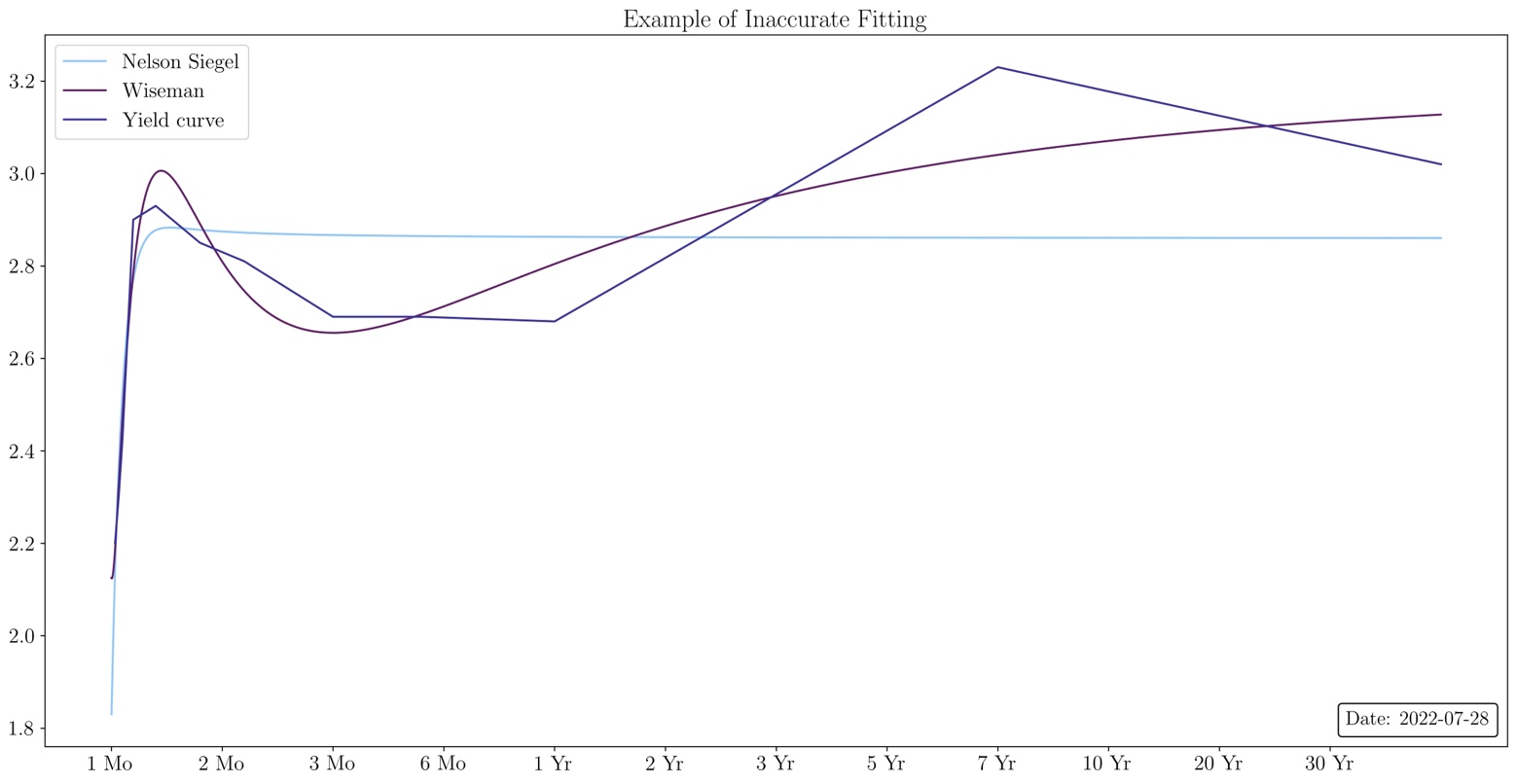
To conclude, we test the residuals of the model by computing the Mean Squared Error (MSE), and we compare them with those of Wiseman (2012). Overall, both models exhibit greater accuracy in 2021, whereas the residuals in 2022 are higher and more volatile. This is probably due to the abnormal shapes of the yield curve this year (see above). Wiseman’s model has consistently lower residuals in the period considered.
Sources
- Cohen, Kramer, Waugh, 1966. “Regression Yield Curves for U.S. Government Securities”.
- Echols, Elliot, 1976. “A Quantitative Yield Curve Model for Estimating the Term Structure of Interest Rates”.
- McCulloch, 1971. “Measuring the Term Structure of Interest Rates”.
- Vasicek and Fong, 1982. “Term Structure Modeling Using Exponential Splines”.
- Nelson, Siegel, 1987. “Parsimonious Modeling of Yield Curves”.
- Litterman, Scheinkman, 1991. “Common Factors Affecting Bond Returns”.
- Adams, Van Deventer, 1994. “Fitting Yield Curves and Forward Rate Curves with Maximum Smoothness”.
- Svensson, 1995. “Estimating forward interest rates with the extended Nelson & Siegel method”.
- Jeffery, Linton, Nguyen, 2000. “Flexible Term Structure Estimation: Which Method Is Best?”
- Hagan, West, 2008. “Methods for Constructing a Yield Curve”.
- Wiseman, 2012. “The Magpie Yield Curve Model at SG”.
- Annaert et alii, 2012. “Estimating the Yield Curve Using the Nelson-Siegel Model: A Ridge Regression Approach”.
- ECB, 2018. “Yield curve modelling and a conceptual framework for estimating yield curves: evidence from the European Central Bank’s yield curves”.


0 Comments