Deep insights into one of the most reliable recessions predictor: the yield curve inversion

Download PDF

Introduction

Economics and the world economy are peculiar for being so unpredictable. The constant involvement of human beings leads them far from being an exact science. Correspondingly, financial markets are even more uncertain, constantly driven by human behaviour. For this reason, the idea that one very simple predictor can forecast with relative certainty the path of the economy is extraordinarily fascinating but, at the same time, heavily debated.

This article dissects what markets consider the best predictor of a future recession: an inversion of the yield curve.

The first part explains the economic intuition behind this event and which curve investors should watch. We then look back at the previous cases and examine what has happened recently. In the central part, we briefly review existing literature and conduct an extended econometric analysis. The results will then be compared to the past ones. Finally, before concluding, we investigate how the stock market performs following an inversion and examine stock return predictability.

Economic intuition

To understand why an inversion of the yield curve predicted all six recessions since 1978 (Fig.1), let’s start with what determines its slope. Starting from a world in which investors care only about returns and not about maturity, in the so-called expectations theory, long-term rates should be equivalent to the average of the short-term rates expected in the future. This, however, cannot explain why we observe a generally positive slope of the yield curve. According to the expectations theory, markets should constantly expect higher rates in the future to motivate a positive slope. Indeed, in reality, investors care about maturity, and they demand compensation for losing capital for a more extended period, the term premium.

Having explained the rationale of a positive slope, let’s see what influences how positive the slope is. We can break down the curve in two parts. The long end is determined by investors’ expectations about inflation and growth in the long term. The short end is mainly influenced by expectations about monetary policy in the near future. Intuitively, when the economy is booming, the yield curve tends to be steep due to an increase in the likelihood of higher short-term rates in the future (this will be reflected in long-term rates). On the other hand, when investors forecast a recession, the yield curve flattens due to expectations of lower rates in the future and excessive tight monetary policy in the short-term.

Despite being an infrequent event,  panic starts to spread among investors when the yield curve flattens so much that it inverts. One explanation for such strong predicting power is that to produce a truly (we will get back to this) inverted yield curve, investors must expect protracted monetary easing by the Fed that only a recession could justify such expectations. Moreover, the yield curve is influenced by more than monetary policy expectations. It reflects market attitudes toward various risks (expressed in the term premium) influenced by economic outcomes too. Therefore, the spread combines a variety of factors and reflects market assessments of the likelihood of a recession in the near future.

Now we get to one of the most heavily debated arguments, does an inverted yield curve cause a recession, or does a recession cause an inverted yield curve? We believe that the truth lies somewhere in the middle. As we said before, it is reasonable to assume that the slope reflects changing expectations about the economy, especially during economic downturns. In addition, in predicting a recession, we believe that the inversion of the yield curve over history has become a somewhat self-fulfilling prophecy.

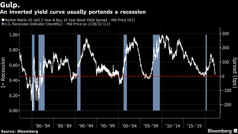
Figure 1: Bloomberg

Which yield curve?

Media and newspapers often exploit the inversion of parts of the yield curve to spread panic and write articles with catchy headlines. In this paragraph, we want to clarify, once and for all, which curve has the highest predicting power.

The most observed curves are four: 3m to 10y, 2y to 10y, 5y to 30y and the so-called “near-term forward spread”, that is, the spread derived from the current three month Treasury bill rate and the implied three-month forward rate in six quarters from now.

We will discard the 5y to 30y curve because it didn’t predict the 2020 recession and ceased inverting almost two years before the 2008 recession. Other curves stayed inverted up to 6 six months before the global financial crisis. Logically, the 2020 recession caused by Covid couldn’t be predicted but all other term spreads were already in negative territory.  Traditionally, academic literature focuses on the 3m to 10y curve, while financial commentators tend to follow the 2y to 10y curve. The “near-term forward spread” gained popularity recently after Engstrom and Sharpe (2018) argued that it might be preferable because it focuses solely on expectations of the near-term path of monetary policy.

Since the 1970s, the three term spreads performed similarly, all entering negative territory ahead of recessions. For a formal investigation of the forecast accuracy of the term spreads, we refer to Bauer and Mertens (2018). Using monthly data from January 1972 to July 2018, they measure the accuracy using the so-called area under the curve (AUC) over the entire sample and over a sample period that excludes the so-called zero-lower bound period (2009-2015) to give the best possible chance to the short-term spread. Overall, they conclude that the 10y-3m spread has the highest predictive power over the entire sample but cannot prevail over the “near term forward spread” if we do not consider the zero lower bound period. The 10y-2y spread, instead, has less predictive power than both the 10y-3m and the “near term forward spread”.

The results of the analysis (Fig.2) are consistent with the findings of Engstrom and Sharpe (2019) (Table 1), which argued that the “near-term forward spread” statistically dominated the 10y-2y spread and that in predicting recessions, the 10y-3m and the near-term spread have almost the same explanatory power. Further analyses were conducted by Engstrom and Sharpe (2019). By including both the near-term spread and the 10y-3m in a single model (Table 1, column 5), evidence showed that all of the information in the long-term spread is already contained in the near-term forward spread. Therefore, we suggest the near-term spread as the best recession predictor following the studies.

Interestingly, on March 21 2022, Fed Chair Jerome Powell conveyed attention to the shorter part of the yield curve. Referring to the first 18 months of the yield curve, “That’s really what has 100% of the explanatory power of the yield curve. It makes sense. Because if it’s inverted, that means the Fed’s going to cut, which means the economy is weak.” In response to a question at the National Association for Business Economics, Powell said.

Finally, It is crucial to underline strong evidence from academic literature that it is appropriate to look at the spread as a recession predictor on at least a monthly average basis.

Figure 2: “Information in the Yield Curve about Future Recession” by Bauer and Mertens

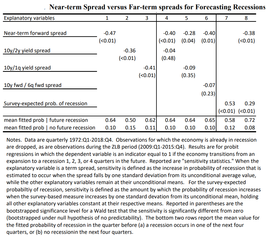
Table 1: “The Near-Term Forward Yield Spread as a Leading Indicator: A Less Distorted Mirror” by Engstrom and Sharpe

Historical analysis

In this paragraph, we will analyse the behaviour of the yield curve during the six recessions that occurred since 1978. It is interesting that historically, recessions were always preceded by Fed tightening (Fig.3). The Fed achieved a “soft landing” only in 1964, 1984 and 1993. Certainly, this contributes to explaining why the yield curve inverted before every recession.

Table 2 summarises the lag between the inversion of the yield curve and the start of the recession. The inversion date is the first negative monthly average observation of the 10y-3m. The average lag between an inversion of the yield curve and the beginning of a recession has been 11-12 months.

Fig. 4 represents the yield curves during all five recessions since 1978 except for the one prior to the 1981 recession because it was so sharply inverted that it would overwhelm the scale of the chart. Generally, before a recession hits, all parts of the curve are clearly inverted. In 2019, however, the curve assumed a strange shape, the 5y-30y part wasn’t inverted, and the 2y-10y reversed for a few days by a few basis points.

During 2019, before the Covid recession, the 3m-10y curve has been negatively sloped for 117 days (3 months with a negative monthly average spread). Surprisingly, the 2y-10y curve was inverted for only three days. Usually, the 2y-10y curve inverts more frequently than the 3m-10y Estrella and Trubin (2006). To put things in context, all the six recessions considered have been preceded by at least three negative monthly average observations (10y-3m spread) in the twelve months before the recession.

However, we don’t know what could have happened if Covid didn’t hit, but we know for sure that this last observation will increase the predicting power of the 3m-10y over the 2y-10y.

Figure 3: Bloomberg

Table 2: Bocconi Students Investment Club

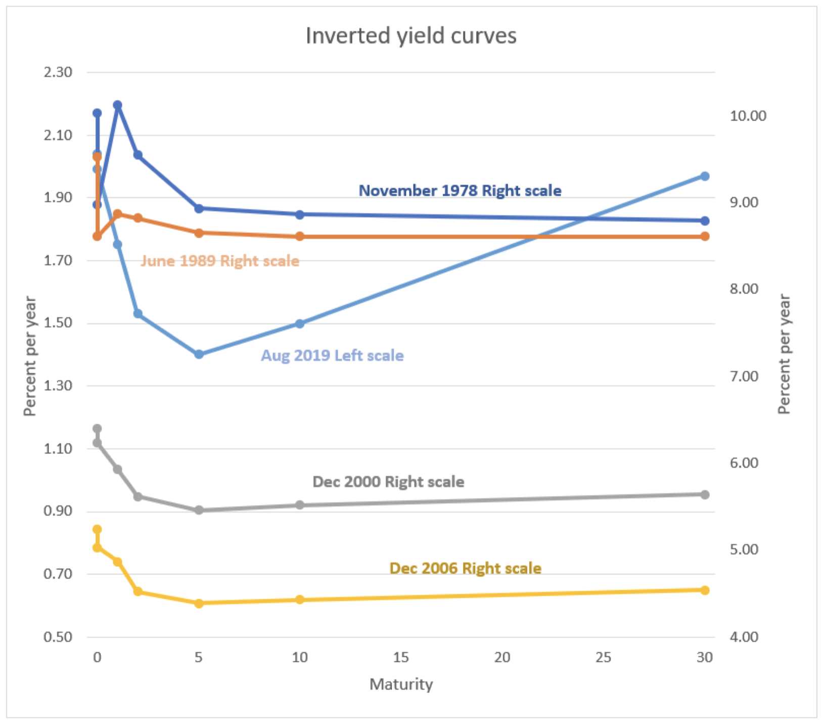
Figure 4: Bocconi Students Investment Club

Where are we?

After having analysed the previous inversions, we now discuss what happened recently.

Inflationary pressure due to supply shortages and the energy crisis has brought the Fed to raise rates for the first time since 2018. Despite the initial reassurance of being only temporary, now markets believe that the Fed is well behind the curve. Market participants are now pricing in another six rate hikes by the end of the year (Fig.5), hypothetically bringing the Target rate to the 250-275 range. Expectations about the Fed Funds Rate path have changed radically in the last six months. According to Bloomberg WIRP, the year-end projection for the FFR went from 0.34% (Sept.30) to 2.35% (Mar.28).

All this has been reflected in the yield curve. On Tuesday, the 10y-2y spread went negative for the first time since 2019 but closed positively (Fig.6). It returned negative numerous times during the remaining trading week but always remained in positive territory at the end of the day. It ceded on Friday, closing negatively at around -7 bps.

At this point, you are probably asking yourself at which level is the 10y-3m or the near-term spread.

Fig. 7 shows the 10y-3m and the 10y-2y spreads together. Two things immediately stand out: first, the recent divergence between the two and second, the little difference between the two paths in the past. We believe that there are three non-exclusive explanations for this: first, the 3-Month Treasury Bill rate prices only what will happen in the next three months, second, the Fed has never kept rates so low, and therefore it is natural for the 10y-3m spread too be so high and lastly, this tightening cycle is relatively faster than previous one. These factors combined debunk what could be sold as “a recession is not coming according to the 10y-3m spread”. If expectations about the FFR are correct, the 3m-10y curve will likely flatten in the following months and this gap will close up.

Going back to the discussion on which spread is the more reliable and recalling that there are evidence that the 10y-2y spread tends to turn negative earlier and more frequently than the 10y-3m spread, we want to conclude the discussion by saying that despite the 10y-3m spread and the near-term spread have higher predicting power, inversion of other parts of the curve, such as the 10y-2y, should also be watched because of their timing advantage. However one should wait for the spread previously discussed to turn negative for an accurate signal.

Figure 5: Bespoke Investment Group, CME Group

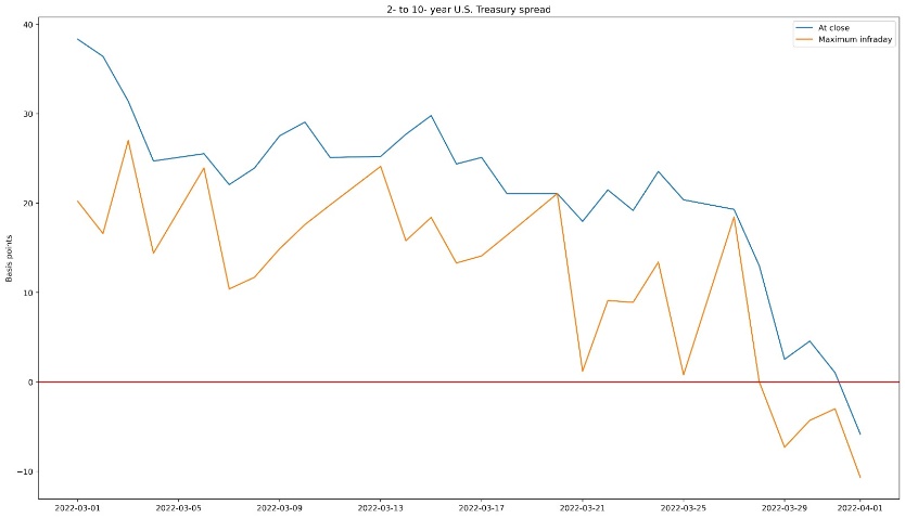
Figure 6: Bocconi Students Investment Club

Figure 7: Bloomberg

Literature Review

After having laid the groundwork for a better understanding of the topic, we now briefly review the paper “The Term Structure as a Predictor of Real Economic Activity” by Estrella and Hardouvelis. The predictive power of the 10Year-3Month Treasury spread on the US GNP is analysed from 1955 to 1988. Recall that the near term spread gained popularity only recently and before that, staff in the Federal Reserve focused on the 10y-3m spread.

First, the authors developed several time-series econometric models (linear and logistic) to explore the forecasting capability of the spread for different time horizons, using both marginal and cumulative economic growth as the dependent variables. Then, they investigated whether extra information is embedded in the spread but is not available in other macroeconomics data (e.g. Federal Funds Rate, Index of Leading Indicator, Annualized Rate of Inflation of the GNP Deflator). Finally, they showed statistical evidence of the predictability of the cumulative economic growth up to 4 years into the future and the marginal quarterly economic growth up to one year and a half in the future using the 10Year-3Month spread. In addition, the regression results suggest the existence of extra predictive power of the yield spread over variables such as lagged output growth, lagged inflation, the index of leading indicators, and the level of real short-term interest rates. However, Estrella and Hardouvelis concluded that backwards-looking performances do not necessarily repeat in the future, especially if policymakers will be using this information to take future actions.

Model implementation

Based on the modern economic theories and the rationale explained above, we can build a linear regression model that relates factors in our economy with the future economic growth:

For our specific case, we will use the Gross Domestic Product as the benchmark for the US economy, and in this first part of the analysis, we will only investigate the explanatory power of the variable 10Year-3Month Treasury Yield Spread. Compared to the research carried out by Estrella and Hardouvelis, this article will analyse the data from 1975Q1 to 2021Q3 and explain the results differences between the current analysis and those obtained by Estrella and Hardouvelis (1955Q1-1988Q4).

US GDP data are reported quarterly. We build two different models to explain the variation of this variable over different horizon. First, we use the cumulative GDP change over period k as our endogenous variable

Then we study the effect of the yield spread impact on the marginal GDP change from period t+k-j to t+k, which is defined as:

Finally, we define our exogenous variable as the difference between the 3Month Treasury annualised yield and 10 Year Treasury annualised yield. However, we are matching a “continuous” time series data with a discrete one; therefore, we use the average quarterly data instead of point-in-time data.

Park and Reinganum showed that point in time data contain systematic biases. In addition, using the quarterly average provides superior predictability power of the variable since it checks the robustness of previous results on the predictive power of the term structure that used only point in time data.

The first regression to consider is the following:

Cumulative GDP change:

We analyse the predictive power of the cumulative economic growth over k periods in the future. Two major issues can affect the consistency of the OLS standard errors in the above-described regression: First, the heteroskedasticity is a big issue, the rate of economic growth change over time, the economy enters in periods of favourable condition and those with critical setup depending on many external factors such as policies, total productive factor, technological development, and other major macroeconomics statistics. Therefore, the variance of the GDP growth rate is not constant over time but changes with the different economic cycles and market regimes. Second, the overlapping exogenous variables used in the regression generates a moving average (serial correlation) error of the order k-1. We implement a HAC error structure to solve these problems, choosing k-1 as our lag period of interest.

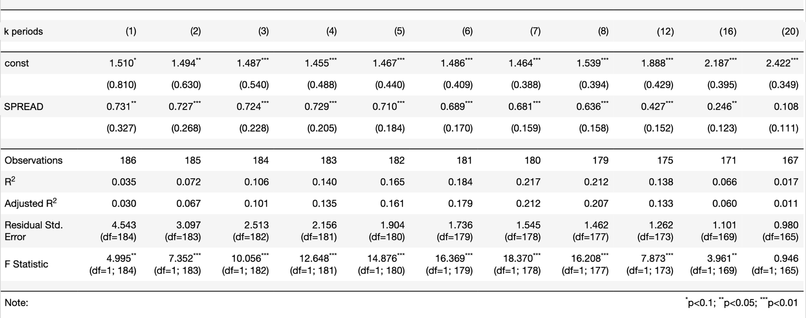
Table 3 – Source: Bocconi Students Investment Club

Using Table 3, we are able to estimate the cumulative economic growth over k periods in the future. For example, if the yield spread at time t is equal to -2,00%, then we will experience zero expected cumulative economic growth in the next 4 quarters (Solve the equation 1.455+0.729*SPREAD0).

The Adjusted represents the percentage of the total variation of the observed dependent variable explained by the model (it provides a measure of how well your independent variable is at explaining the variable of interest). The predicting power of the model is maximum for 6, 7 and 8 periods ahead (in these cases, the regression explains respectively 17.9%, 21.2%, 20.7%). Comparing the results of Table 3 with those obtained by Estrella and Hardouvelis back in 1991, it is possible to quickly recognise a drop in the explanatory power of the yield spread and its impact on economic growth (Lower Betas and Lower Adjusted ). Studies in recent years have shown that many economic and historical reasons can be employed to explain this phenomenon (e.g. the increasing number of investors and policymakers use yield spread to take future actions, decreasing term premiums over the years, etc.). We will cover and discuss better these rationales in the next section.

Moving on to our second regression, we construct:

Marginal GDP change:

In this setting, we analyse the marginal j periods economic growth for k quarters in the future. The econometric issues found in the first regression also persist here. The heteroscedastic structure of errors and the overlapping exogenous variables, which generates a moving average problem of the order j-1, must be solved; therefore, we adopt the same methodology described above where the adjustments are necessary.

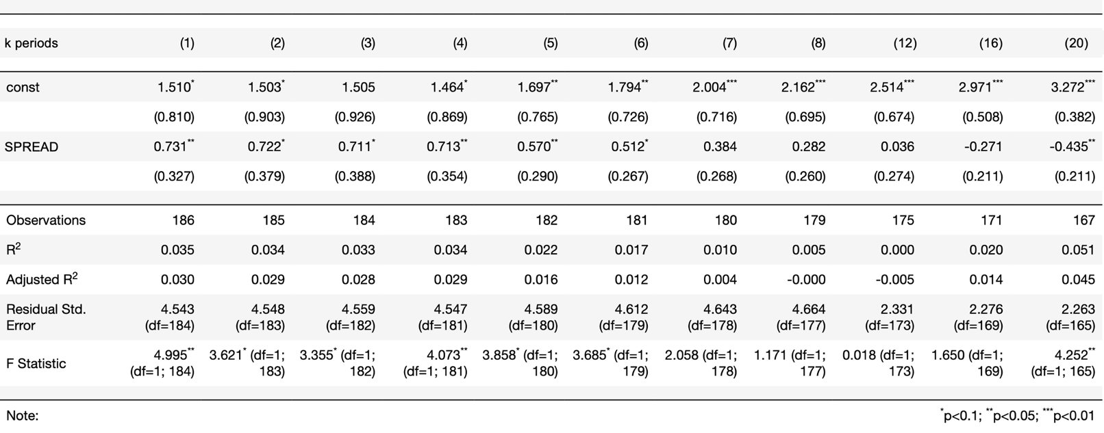
Table 4 – Source: Bocconi Students Investment Club

Using Table 4, we can calculate the necessary yield spread to obtain an expected negative economic growth for two consecutive quarters (economic recession). For example, if the yield spread at time t is equal to -2,98%, then we will experience -0.66% (1.464+0.713*(-2.98)=-0.66) expected marginal economic growth for the quarter 4 and 0% (1.697+0.57*(-2.98)0) expected marginal economic growth for quarter 5.

The variable 10Year-3Month yield spread is statically significant at predicting the marginal economic growth until the quarter in the future. Although the overall predictive power of the model is extremely low, its highest Adjusted are found in the first 4 periods (in these cases, the model explains respectively 3%, 2.9%, 2.8% and 2.9% of the variability of the independent variable); comparing the results of Table 4 again with those obtained by Estrella and Hardouvelis back in 1991, we notice similar differences to those we found in Table 3 (Lower Betas and Lower Adjusted ), but this time, the percentage reduction of the Adjusted is more remarkable.

Analysing Tables 3 and 4, the overall higher Adjusted in Table 3 suggests higher reliability of the cumulative economic growth prediction model compared to the other one. To explain the rationale behind this pattern, we take into consideration the main objective of the Federal Reserve’s actions: promote maximum employment, stable prices, and moderate long-term interest rates. The yield curve spread reflects partially future monetary policies expectations. Employment, inflation and long term interest rates fluctuate over time (over different quarters) in response to various economic and financial shocks (Low practicability power of marginal economic growth model). Therefore, the central banks play an essential role in stabilising the economy and achieving its predetermined long term objectives (High practicability power of cumulative economic growth model). Moreover, in the cumulative economic growth model, the increasing pattern of the Adjusted for higher periods compared to the lower ones is justified by policy lag since it takes time for a policy to achieve its intended objective.

If the marginal economic growth model is a poor predictor of downward economic cycles, as shown in Table 4 and Figure 8 (especially in certain periods, e.g. 1994 – 1999). What solution can be implemented to predict the probability of a future economic recession (negative economic growth for 2 or more consecutive quarters) more precisely? The logistic model could be a valuable solution to this problem.

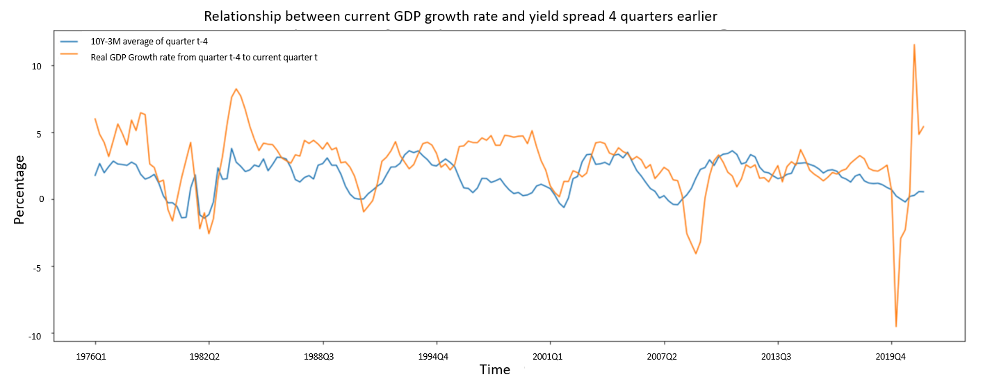
Figure 8: Bocconi Students Investment Club

We construct the third regression model to study the probability of recession at time t+k given the yield spread of the quarter t+k-j:

Where the function is the inverse of a logit function:

This nonlinear regression model provides an accurate relationship between the recession data given by the National Bureau of Economic Research during 1975Q1 – 2021Q3 with the 3Month-10Year Treasury yield spread. Here again, the heteroscedastic structure of errors and the overlapping j exogenous variables are adjusted accordingly using the HAC error structure. We consider 8 different time horizons k (from 1 to 8) for our 8 different models, and we always select j to equal 1.

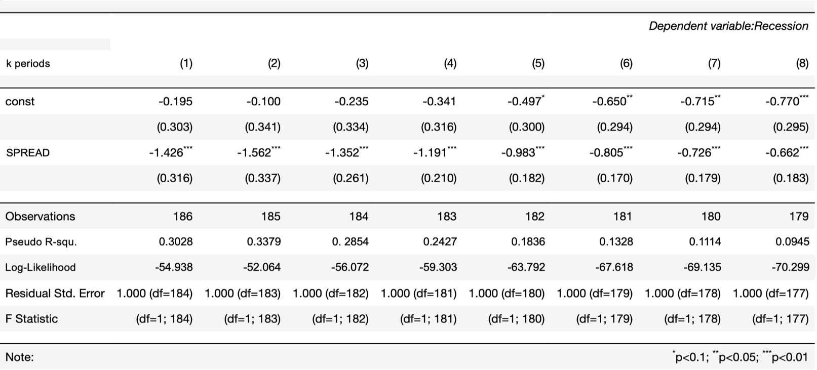
Table 5: Bocconi Students Investment Club

For every analysed period k, the is negative, meaning that the lower the spread is, the higher the probability of a recession. Another interesting trend described in the table is the increasing value of over longer time horizons k. This means that under the same market condition and same yield spread, the probability of recession predicted by this variable is, on average, higher in the short term than in the long term (for negative values of spread). To understand this phenomenon, we recall again the idea of the yield spread as an expectation of future economic growth; historically, the fixed income market has been highly efficient in pricing future macroeconomic expectations; therefore, market participants have kept adjusting the yield curve according to future predictions way ahead of the coming quarters. Therefore, the yield slope price in the possibility of a future recession long time before it actually happens.

The Pseudo R-squared values reported by the models in Table 5 indicate that the spread has a very strong forecasting capability on the probability of future economic conditions; indeed, the models with k=1,2 and 3 explain the 30.28%, 33.79% and 28.54% of the variance of the dependent variable, respectively. When k=2, the model has the highest predictive power. To visualise the relationship graphically, we plot the yield spread data from 1975Q1 to 2022Q1 and predict the probability of recession from 1975Q3 to 2022Q3.

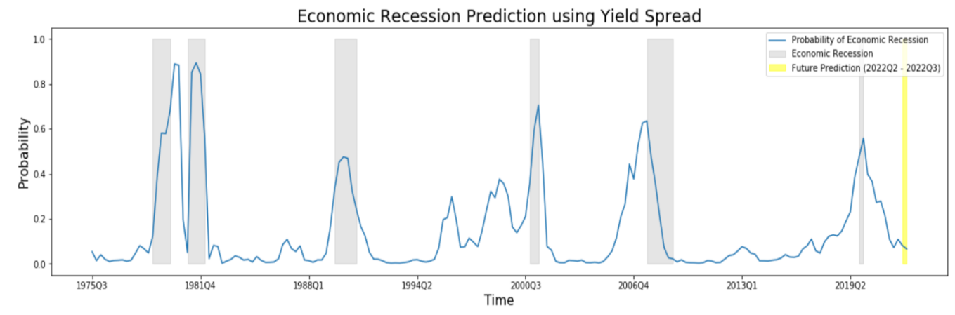
Figure 9: Bocconi Students Investment Club

Historically, the 10Y-3M Treasury spread has shown great reliability at predicting economic recessions for 2 quarters ahead. Although some recent developments suggest a possible economic downturn in the near future, our model still produces a very low probability of economic recession in the 2 quarters ahead (8.14% for 2022Q2 and 6.58% for 2022Q3). A possible limitation of our estimates can be found in the limited data we used as our regressor. The narrowing of the yield spread has started recently, and their effects in our model are negligible because we consider the average quarterly data as our exogenous variable.

To better estimate future probability over a longer horizon (estimating one more quarter ahead), we use Forward rates 3M3M and 3M10Y. The forward average yield spread for the next quarter (2022Q2) is 1.135%; therefore, using the parameters of the model with k=2, the expected probability of economic recession in 3 quarters is 13.31%. Currently, according to the model, the risk of an economic downturn is still very contained; however, the market participants are still pricing in the interest hikes expected for this year, inflation is running hot, and on March 21 2022, Powell explicitly stated that “inflation is much too high” and he implied that Federal reserve would take tough actions to match the inflation expectation with the long term objective of 2%. Most analysts expect a steady increase of 3-Month interest rate along with the Fed Funds Rate since both have been strictly correlated (0.99) over the years.

Figure 10: CME Group

Figure 10 illustrates the Fed Funds Rate expectation for the meeting of 14-Dec-2022. With a probability of 87.1%, it will fall in the range of 225-300bps. Suppose that the 3Month interest rate will be priced similarly to the Federal Funds Rate, while the 10 Year Treasury will increase slower and range around 250-300bps. Then expected future probability of recession based on different spreads are (using the logistic model with k=2 in Table 6):

Table 6: Bocconi Students Investment Club

Finally, we move on to our last regression. The most important question to investigate is whether the yield spread includes information not contained in other statistics. The current monetary policy has a direct impact on the yield spread. If the yield curve slope embeds additional information, then policymakers and investors can exploit it to opt for even better decisions. To statistically test this hypothesis, we include one additional variable among these in our model: Real Federal Funds Rate, Effective Federal Funds Rate or 3-Month Treasury yield (the result is similar no matter what statistic is chosen). We will use the Effective Federal Funds Rate (FFR) for convenience. The regression calculates the cumulative economic growth over k periods using two independent variables:

Cumulative GDP change:

One issue may emerge from the above regression. The correlation between FFR and SPREAD (-0.44 over the analysed period) may create the problem of inconsistent estimators. But do we have to be worried in our case? First, suppose the estimated coefficients are statistically significant even if they embed high variance, this does not affect our conclusion because it means that in the absence of that high variance, the exogenous variables are still statistically significant at estimating the endogenous one. Second, suppose the estimated coefficients are not statistically significant in the presence of inconsistency, in that case, we cannot conclude that the analysed independent variable has no explanatory power because the high correlation problem may be the cause.

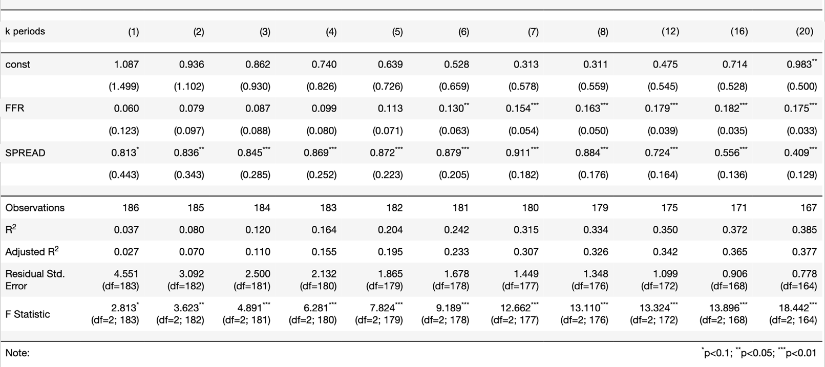
Table 7: Bocconi Students Investment Club

In this case, we do not have to worry about the second scenario we mentioned before, because according to our model, the yield spread is statistically significant at explaining cumulative economic growth for about 5 years even if in the presence of possible collinearity problem.

We can distinguish two components in the 10Y-3M spread, the short end yield (strictly correlated with the FFR) and the long end one. Through the regression results, we can conclude that even if the long end component always fluctuates around its mean, it still embeds predictive power over the future economic growth in the short term (up to 5 years).

Counterargument

Going back to the initial question, our models’ results indicate that the yield slope is a good predictor of cumulative economic growth. But, if we compare our results with those obtained by Estrella and Hardouvelis in 1991, they are slightly different; it seems that the forecasting capability of the yield spread has decreased over time by showing lower beta and lower Adjusted .

Among the factors that influence the yield slope we have already described in this article, we dive deeper into one decisive component, the term premium. The term premium refers to the additional compensation granted for holding long-term bonds over short-term bonds. If the term premium is negative, investors are willing to pay additional money to hold long-term maturities; on the contrary, if the term premium is positive, investors want to receive extra payment to keep long-term assets. Suppose everything remains constant; the decrease in term premium could cause yield curve inversions more probably and frequently even if the risk of negative economic growth over k period has not increased at all. The chart below gives an intuitive way to think about this relationship.

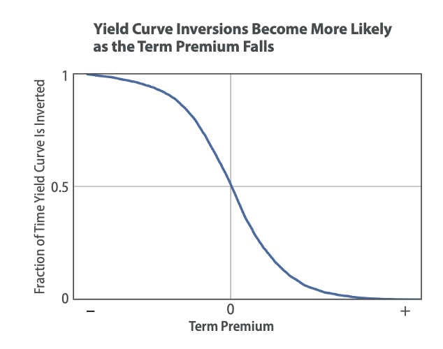
Figure 10: Federal Reserve Bank

The change of the term premium is associated with the change in the demand and the perceived riskiness of the underlying asset. The dominant threats that may shift an investor from holding a 10 Year Treasury are the unexpected inflation risk and unstable economic growth over the years. Observing the studies conducted between the 70s and the 80s, the term premium skyrocketed as the fear for inflation climbed. But since then, these concerns have eased, and bondholders have been more willing to accept lower compensation for bearing inflation risk.

The decrease of the term premium of the 10Year Treasury over the last 3 decades has resulted from the increasing reliability of the Fed at maintaining stable long term inflation objectives and stable economic growth by adopting massive bond purchase programs. Lower coefficients obtained by our models with respect to those obtained by Estrella and Hardouvelis in 1991 may be explained by the decreasing term premium over the years. Estrella and Hardouvelis analysed data from 1955 and 1988; they included a period of structural economic change in the US economy. Central bank policies, the abandonment of the gold standard and market psychology contributed to one of the highest inflation rates periods in the US economy. Surging term premium has enabled a strong predictive power of their models whenever yield slope decreases, and consequently, their results showed higher Adjusted and higher Betas.

Moreover, advanced foreign economies such as Japan and Germany have shown negative 10Y bond yields in recent years. This phenomenon could have caused a spillover effect on the US Treasury by attracting more foreign investors, who wanted to safeguard their money in the US economy, and as a consequence putting downward pressure on the long term end of the yield curve.

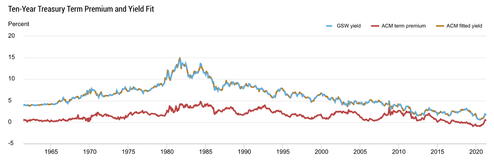
Figure 11: Federal Reserve Bank of New York

Forecasting stock market performance with the term spread

At the beginning of the article, we mentioned that financial markets are even more uncertain than the economy. Forecasting recessions one year in advance is proof of the impressive predictive ability of market participants. But can they do better? In other words, is it possible to improve market performance by looking at the term spread?

A recession has a massive impact on the stock market. Earnings expectations are revised dramatically, investors’ confidence plummets, and as a consequence valuations suffer. Therefore, intuitively, an inversion of the yield curve should also hurt stock market performance.  However, the stock market does not respond right away when a yield curve inverts. Despite the brilliant record of the predictor, most of the time, investors tend to be sceptical at the initial inversion date. Therefore, It is difficult to study the relationship between the two due to the variation in the lag between the three events (yield curve inversion, stock market decline and recession). For this reason, results could vary significantly according to which inversion date and period return one picks.

Table 8: Bocconi Students Investment Club

Table 8 illustrates the performance of the S&P 500 at different points in time, starting from the inversion date of the 3m to 10y curve. Here, differently from Table 2, the inversion date is the first inversion and not the first average negative monthly observation. The dates in yellow represent the range in which the recession began. Excluding the distinct case of 1978, in all other cases, the market eventually collapses. Exiting the market too soon can imply missing significant gains, but if one stays invested and tries to time too aggressively the market, that can result in huge losses of both time and capital.

Moreover, Table 9 from Engstrom and Sharpe (2019) shows the result of their investigation. Annual stock returns are regressed on interest spreads (quarterly average preceding the annual return period) by including a dummy for when the spread is negative. Looking at the results for the near term spread (Table 9, column 1), the coefficient on the spread level is statistically insignificant, but what is remarkable is the coefficient of -22 on the dummy. In other words, when the near-term forward spread is negative, the market has a 22% lower average excess return. Columns 2 and 3 show the results for the 10y/2y and the 10y/3m spread. None of them has any predictive power even though the 10y3m dominates the 10y2y. Column 5 combines the more conventional predictors such as the short interest rate and the earnings yield to the near-term forward spread. The inversion dummy is now even more significant, and the adjusted R-squared equals to 0.28.

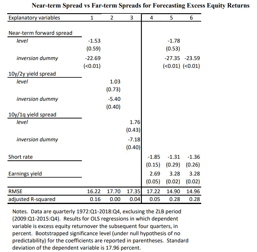
Table 9: “The Near-Term Forward Yield Spread as a Leading Indicator: A Less Distorted Mirror” by Engstrom and Sharpe

These results suggest that the term spread could improve the performance of a buy-and-hold portfolio if taken into consideration in a portfolio strategy.

Engstrom and Sharpe (2019) test a strategy in which the market is held in any given quarter if and only if the near-term spread was positive during the preceding four quarters. Otherwise, the portfolio holds Treasury Bills. Figure 12 shows the cumulative log returns to the market timing strategies. The asterisks illustrate the period when the strategy keeps investors out of the market. The strategy yields an average quarterly return of 0.55% higher than the buy-and-hold, statistically significantly lower volatility, a higher Sharpe ratio and the max drawdown is significantly lower (-27.85% vs -46.33%).

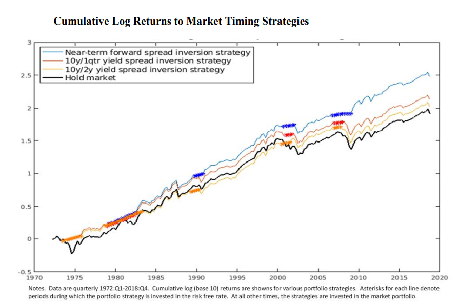
Figure 12: “The Near-Term Forward Yield Spread as a Leading Indicator: A Less Distorted Mirror” by Engstrom and Sharpe

Conclusion

To conclude, we summarise the main concepts and findings of this article:

1. The yield curve contains additional information compared to the monetary policy expectations, it reflects market assessments of the likelihood of a recession in the near future
2. The two most powerful predictors are the 10y-3m and the “near-term forward spread”, recent studies show that the latter contains all the information present in the former
3. The average lag between an inversion of the 3m to 10y yield curve (negative monthly average observation) and the beginning of a recession has been 11-12 months
4. The 10y-2y spread closed negative on Friday and the gap with the 10y-3m will close up in the following months
5. The linear regression model returns the highest predicting power for cumulative growth over 6, 7 and 8 periods ahead
6. A -200 bps implies zero cumulative economic growth over the next four quarters
7. The cumulative economic growth prediction model is much more reliable than the marginal one
8. The logistic model is very powerful in predicting recessions (with k=2, Pseudo R-squared = 33.79%)
9. If we end up with a -50 or -25 bps spread by then end of the year the model gives respectively 66.40% and 57.20% probability of recession in 2023Q2
10. A Near-term spread portfolio strategy is a very simple strategy that drastically outperformed the market over the history

References

Eric Engstrom and Steven Sharpe, February 2019, “The Near-Term Forward Yield Spread as a Leading Indication: A Less Distorted Mirror”, Federal Reserve Board

Renee Haltom, Elaine Wissuchek, and Alexander L. Wolman, December 2018, “Have Yield Curve Inversions Become More Likely?”, Economic Brief, Federal Reserve Bank of Richmond

Michael D. Bauer and Thomas M. Mertens, August 2018, “Information in Yield Curve about Future Recession”, FRBSF Economic Letter

Eric Engstrom and Steven Sharpe, June 2018, “(Don’t Fear) The Yield Curve”, Federal Reserve Board

Michael D. Bauer and Thomas M. Mertens, March 2018, “Economic Forecasts with the Yield Curve”, FRBSF Economic Letter

Arturo Estrella and Mary R. Trubin, August 2006, “The Yield Curve as a Leading Indicator: Some Practical Issues”, Current Issues in Economics and Finance, Federal Reserve Bank of New York

Dusan Stojanovic and Mark D. Vaughan, October 1997, “Yielding Clues About Recessions: The Yield Curve as a Forecasting Tool”, Federal Reserve Bank of St. Louis

Arturo Estrella and Gikas A. Hardouvelis, June 1991, “The Term Structure as a Predictor of Real Economic Activity”, The Journal of Finance