An Overview of Now-casting Methods

Download PDF

Introduction

Now-casting methods are a class of forecasting models originally used in meteorology, and that later found useful applications in economics and finance. The first paper that generalizes the use of now-casting methods in economics is Giannone, Reichlin, and Small (2008). The idea of now-casting is that high-frequency variables can be used to provide a timely forecast of a low-frequency target variable, and that the forecast can be revised whenever a new value for the high-frequency variables is released. The high-frequency variables can combine “hard” data (e.g., industrial production) and “soft” data (e.g., surveys), which can be released asynchronously at different frequencies.

Now-casting models are particularly useful in economics since several economic indicators such as GDP are only available with a significant delay. For instance, GDP is published in US and UK one month after the end of the reference period, and the in the EU the lag is even longer by 2/3 weeks.

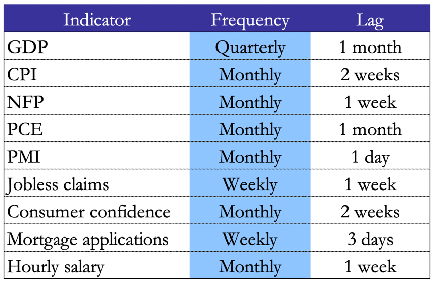
Table 1. Economic Indicators in the US

Now-casting models must handle data which is 1) released at different frequencies 2) released with different delays and 3) high-dimensional. A class of models that satisfy these criteria has been identified by the literature. It includes, but it is not limited to, dynamic factor models, mixed frequency VARs, bridge equations and ML models.

State Space Models

State-space representation models are described by a system of two equations: measurement equations that link a latent state process to the low-frequency target variable, and transition equations that describe the inner dynamics of the latent state process. State-space models allow the use of Kalman filter, which can manage missing data (due to asynchronous data release or missing data collection) and mixed-frequency data. Moreover, if the high-frequency features are numerous and exhibit significant co-movement, then it is appropriate to reduce their dimensionality through Principal Components Analysis, following Giannone, Reichlin, and Small (2008).

We will now introduce the mathematical formalization of now-casting trough state-space models. The aim is to forecast a low-frequency target variable using the information contained in the set , where is a time index. The low-frequency variable can be seen as a high-frequency variable with periodically missing observations. In this way the model dynamics can be specified at a high-frequency. For a variable , we define its counterpart at an observation frequency . Clearly, if the new observation frequency is higher than the original one, the variable will have periodically missing observations.

The latent state representation for the vector is the following:

• Measurement equation: , where ,
• Transition equation: , where .

is the vector of low-frequency observed variables and is the latent state vector, which can be expressed through factors (dynamic factor models). and are the coefficients governing the two equations, while and are the residual terms. Both the coefficients and residuals’ covariance matrices can be time-varying.

The Kalman filter and smoother provide the expectation of the state vector conditioned on the information set, together with the precision of this conditional expectation:

• Conditional expectation: ,
• Precision: .

Modelling the Surprises

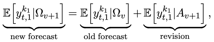
One of the main advantages of now-casting is that it allows to extract a model-based surprise or unexpected component of a newly released high-frequency data. Since the changes in the forecast of the target variable can be expressed as a weighted average of the surprises in the high-frequency variables, the model also allows to extract weights for the high-frequency variables. Given an information set that expands when moving from index to due to a new release:

where is the unexpected component of the new release, that is the component of which is orthogonal to the information contained in . We think about as the surprise or “news”. By developing the expression above, we can obtain:

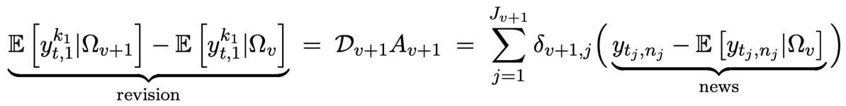
where is the vector of weights of the news. To sum up, the revision is decomposed as the weighted average of the news in the latest release.

Bridge Equations and ML Models

Bridge equations models are a now-casting tool used by central banks to obtain early estimates of GDP. Contrary to state-space models, bridge equations do not jointly model the variable of interest and the predictors (previously referred to as state vector), therefore it is not possible to extract a model-based surprise with these models.

In bridge equations the mixed frequency model is solved by aggregating the high-frequency variable to match the frequency of the target variable. The model is described by the equation below, which is estimated through OLS: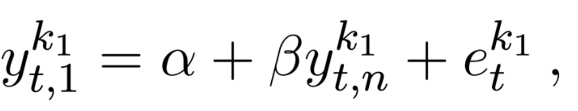

where is the aggregated predictor.

More recently, several Machine Learning (ML) methods have been used in the context of now-casting. Kant et al. (2022) find that, since the GFC, ML models have been more accurate than traditional dynamic factor models across different forecasting horizons, because they manage to find the right balance between “soft” data (e.g. surveys) and “hard” data (e.g. production), whereas dynamic factor models tend to overweight “hard” data.

Kant et al. (2022) test different ML models to predict the Dutch GDP with a set of 83 macroeconomic and financial variables. The models used are LASSO, adaptive LASSO, Ridge, random subspace methods and random forests with Shapley values. After analysing several papers that employ ML models, Kant et al. (2022) conclude that random forests are the ML models which achieve the best accuracy results across different countries and target variables, namely, GDP, inflation and other macroeconomic series.

We will now describe the functioning of random forests algorithms. Decision trees are algorithms that make predictions by posing a series of tests on given data points. This process can be represented as a tree, with the non-leaf nodes of the tree representing these tests, and the leaves of the tree representing the values to be predicted after descending the tree (performing the tests). The tests can be based on an entropy maximisation criterion or on a squared error minimisation criterion, and they can take the simple form: “is feature j of this point less than the value v?”. Random forests are a class of ensemble learning methods that combine the predictions of many decision trees through majority voting or averaging to reduce the variance of the predicted values while maintaining the same expected value. Moreover, the different decision trees are trained in a randomized way so that the correlation between them decreases. Another important feature of random forests is that their results can be interpreted through the Shapley values, which are a tool to decompose the contribution of each feature to the final forecast. This is fundamental whenever ML models need to be incorporated into a decision-making process.

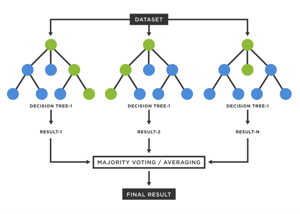
Figure 1. Random Forest, Source: TIBCO Software

Empirical Studies on Now-casting

The literature concerning now-casting in economic and financial applications is vast and quickly growing. However, now-casting is still a relatively young field of econometric research with the first papers being published around 15-20 years ago. While influential studies comparing methodologies such as [1] and [2] have been published, no consensus has yet been reached on how to best apply these methods empirically. Stundziene et al. (2023) [4] give an up-to-date and broad overview of empirical work in now-casting. Due to the vastness and heterogeneity of the field, this section of the article will be largely based on [4].

To start off, we will present some empirical facts on research on now-casting compiled by Stundziene et al., based on their analysis of 193 papers. They find that the number of articles being published on now-casting is increasing over time, with a significant number of papers starting to be published after the Eurozone crisis. Moreover, now-casting research is more prevalent in Europe than in the US/North America and only a small portion of papers cover Asia and other regions. The largest fraction of papers investigates now-casting techniques for GDP but some papers also now-cast labour market statistics, inflation rates, and other variables. Lastly, a wide range of now-casting methods are used, the most prevalent of which have been covered in the previous sections of this article. We will delve somewhat deeper into this last observation.

In general, it has been found that dynamic factor models (DFMs) tend to outperform naïve models such as ARMA or VAR models. This type of model is also by far the most prevalent model used in academic research. MIDAS models (not covered in this article in detail) are the second most used models and have been shown to potentially outperform even sophisticated DFMs. Bridge models are also commonly used and can outperform DFMs. The best performance, however, is most often achieved when multiple models are combined. Lastly, Machine Learning models are present in a small but increasing share of papers and have been shown to outperform DFMs and other naïve models.

The main problems of now-casting pertain to the quality and, most importantly, the availability of real-time data. While studies have traditionally focused on conventional datasets such as oil prices, bank assets, interest rates, and export and import figures, there is a growing interest in using so-called alternative datasets in now-casting applications. The most prevalent alternative datasets are textual data from blogs, news, and social media platforms as well as trend data from search engines. The potential advantage of alternative datasets is that they are either available in a quasi-continuous fashion (textual data) or in near-real time (search engine data). Richardson (2018) [5] provides an overview of potential use cases and problems of using such alternative datasets.

The author documents that there is no clear dominance of alternative datasets over conventional ones or vice-versa. In fact, it is shown that purely statistical approaches (i.e., approaches that do not incorporate alternative datasets into economic theory) often do not outperform traditional methods while those that do incorporate alternative datasets into economic theory tend to outperform traditional methods more often. Still, there are some major challenges with using these datasets. The main problems are that the data can be 1. very noisy, 2. subject to qualitative decisions made by researchers (e.g., the choice of keywords to filter for), and 3. only available in short samples.

To sum up, the empirical field of now-casting is still developing and no clear standards have been set for which methods or datasets to use. On the one hand, this gives researchers the freedom to explore new, alternative now-casting methodologies while, on the other hand, making research less comparable. Nevertheless, we believe that now-casting can provide valuable input both for financial markets participants as well as regulators. As a short case-study we will now give a quick overview of an important and influential now-cast of US GDP: GDPNow.

GDPNow

The GDPNow now-cast of quarterly US GDP growth is one of the most well-known now-casts. It is calculated and published by the Federal Reserve Bank of Atlanta and largely draws on the methods outlined in [1]. The specific methodology for the now-cast is outlined in [6] and can be summarized as a Bayesian VAR model that is augmented by bride equation regressions. With this model, forecasts of all components of GDP are made and combined into a total GDP forecast.

In general, the GDPNow now-cast has been quite accurate, and the accuracy improves over time. In the following two graphs, GDPNow now-casts are compared with the Bureau of Economic Analysis (BEA) advance estimate of GDP which is released about 25-30 days after the end of a quarter.

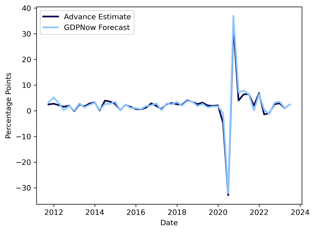
Figure 2. Now-cast Accuracy of GDPNow, Source: Atlanta Fed, BSIC

As one can see, the most recent estimate of quarterly GDP as computed by GDPNow is very close to the actual Advance Estimate by the BEA. In fact, over this time-period, the RMSE only was 1.19 which is heavily skewed upwards by quite a large miss during the first quarter of 2020, i.e., when the Covid-19 pandemic hit the country.

Figure 3. Average GDPNow Error over Time, Source: Atlanta Fed, BSIC

This graph neatly shows that the average error when now-casting quarterly GDP is strictly decreasing as the actual release of GDP figures comes closer which shows the efficacy of having frequently updating now-casts. Furthermore, the average error of now-casts even 1-2 months out from the release is still low when considering that GDP is a notoriously hard variable to forecast accurately.

References

[1] Giannone D., Reichlin, L., and Small, D.H., “Now-casting GDP and Inflation”, 2008, ECB Working Paper Series

[2] Giannone D. et al., “Now-casting and The Real-time Data Flow”, 2013, ECB Working Paper Series

[3] Kant D. et al., “Now-casting GDP Using Machine Learning Methods”, 2022, De Nederlandsche Bank

[4] Stundziene A. et al., “Future directions in now-casting economic activity: A systematic literature review”, 2023, Journal of Economic Surveys

[5] Richardson P., “Now-casting and the Use of Big Data in Short-Term Macroeconomic Forecasting: A Critical Review”, 2018, Economie et Statistique / Economics and Statistics

[6] Higgins, P., “GDPNow: A Model for GDP ‘Nowcasting’”, 2014, Federal Reserve Bank of Atlanta Working Paper Series