Barbell and Bullets: Fixed Income Portfolios for Turbulent Times

Download PDF

Introduction

Fixed income investments allow investors to generate steady cashflows in the future, diversify equity exposure, and lower portfolio volatility.

Current inflationary pressures, tighter monetary policy, and concerns about the prospect of rising interest rates are making investors question how strategic exposure to fixed income securities can help lower risks.

In this article, we present the Barbell strategy and discuss how to navigate this highly volatile market environment while limiting downside risks. Before we do so, we review the concepts of DV01, duration, and convexity, presenting their essential role in fixed-income risks management. Finally, we propose a trade idea using the above-mentioned strategy. We will seek to limit sensitivity to macroeconomic sources of risk without giving up too much return.

Theoretical background

DV01 & duration

DV01 measures the dollar change in the value of a security for a one-basis point change in yield. Other measures of interest rate sensitivity, Macaulay duration, and Modified duration, measure respectively the weighted average time until cash flows are received and the percentage change in the security value for a unit change in rates. Mathematically, DV01 and Modified Duration are defined by:

It is important to note that since DV01 is based one-basis point change, which is 0.01%. Dividing it by 10000, we are rescaling from 100% to 0.01%, equivalent to one basis point.

From now on, we’ll use duration only to refer to Modified duration, since it is a more precise measure of interest rate sensitivity. Formally, modified duration is a semi-elasticity, the percent change in price for a unit change in yield, rather than an elasticity, which is a percentage change in output for a percentage change in input.

The negative signs that define both DV01 and Duration show the negative correlation between rates and prices. Mathematically, these two concepts are associated with the tangent line at a particular yield and are therefore proportional to the derivative of the price function.

Source: IFT

Convexity

As shown in the figure above, as the yield changes considerably from a particular reference level, DV01 and duration become poor estimates of price change, i.e., DV01 declines relatively moderately as rates rise, and increases relatively rapidly as rates decline. Convexity measures interest rate sensitivity change with the level of rates. Mathematically, convexity is defined as:

Using a second-order Taylor formula of the price-rate function with respect to interest rates, we can derive the following approximation for the price change after an infinitesimal change in yield:

As yield fluctuations become bigger in either direction, the effect on price changes has a more significant impact due to positive convexity, which increases gains as yields go down and limit losses as yields go up. Conversely, negative convexity limits gains as yields go down and enhance losses as yields go up.

In the investment context, choosing among securities with the same duration expresses a view on interest rate volatility. Selecting very positively convex security is essentially a long volatility position.

A note on convexity and embedded optionality

The higher a bond’s time to maturity, the greater its sensitivity to interest rates changes. What happens when we deal with option embedded bonds?

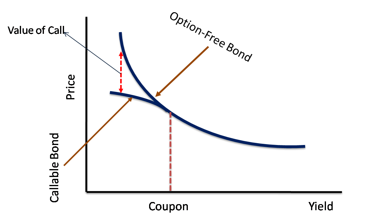
Callable and puttable bonds have embedded options for possible early redemption. Interest rate risks behave differently in these 2 cases. The callable bond can be represented as a combination of a long position in a non-callable bond and a short position in a call option.

A callable bond shows positive convexity for positive changes in interest rates (as a noncallable bond) and negative convexity for negative changes. When rates go down, the value of the embedded call option increases (because the issuer has a higher incentive to exercise the right and refinance at a lower cost), and option-free bond prices increase, thus the price of a callable bond will not rise as much as its comparable non-callable bond (recall that we subtract the value of the optionality from the price of the noncallable bond because optionality belongs to the bond issuer, not the bond holder). Therefore, it exhibits negative convexity for rate decreases.

Source: Fintelligents

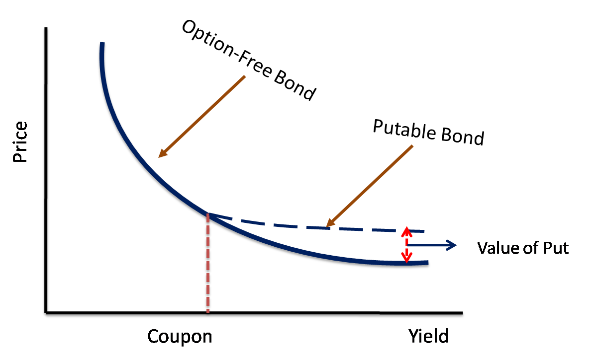
A puttable bond, on the other hand, can be represented as a combination of a long position in a non-callable bond and a long position in a put option since the bond holder has the right to demand repayment of the principal before maturity.

A puttable bond exhibits positive convexity for positive rate changes and negative convexity for negative changes. As interest rates decrease, the bond exhibits a price/yield relationship similar to option-free bonds. In the opposite scenario, when interest rates increase, the value of the put option increases while the price of a nonputtable bond falls, thus the price of a puttable bond will not decrease as much as a corresponding nonputtable bond.

Source: Fintelligents

Portfolio properties

The dollar value of a portfolio is the sum of the value of its components, and the derivative of a sum is the sum of single derivatives, thus we can derive:

If we divide both members by -10000, we derive the portfolio DV01 as the sum of individual securities’ DV01s:

Start again from the sum of derivatives, divide both sides by -p; on the right side, multiply and divide each factor by , and we obtain:

The duration of a portfolio equals the weighted sum of individual durations. Convexity is derived in the same way, taking the sum of second derivatives, giving:

Bullet vs Barbell Strategy

The barbell strategy represents one of the most appealing approaches to fixed income investing when the markets are turbulent and the macro scenario uncertain. This technique reduces investors’ exposure to interest rate risks and helps them navigate rising rate environments, such as the one we currently find ourselves in.

The strategy combines long-maturity with short-maturity securities. The portfolio is created to replicate the duration of a bullet portfolio that concentrates on intermediate-maturity bonds.

Duration increases linearly with maturities, while convexity increases with the square of the maturities. Therefore, while exhibiting the same duration of a bullet, the barbell promises greater convexity because it offers exposure to the maturities where the price-yield relationship exhibits the greatest curvature. More generally, for a given duration, convexity is higher for more dispersed cash flows. For example, a coupon bond has greater convexity than a zero-coupon bond with the same duration.

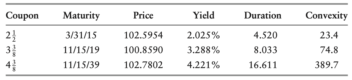
Of course, the barbell also presents a major disadvantage: a normal yield curve presents a negative concavity, therefore, according to Jensen’s inequality, the weighted average yield of the barbell strategy is generally lower than the bullet’s. In short, we can interpret this spread as the cost of taking additional convexity. Investors believing that rates will be particularly volatile will prefer a barbell strategy, otherwise, they would favor the bullet one. Obviously, calculations must be carried out to assess how volatile rates have to be for the barbell portfolio to outperform., i.e., on May 28, 2010, an investor is considering the purchase of three U.S Treasury Bonds.

Source: Fixed Income Securities [1]

To reproduce the duration of the 10-year bond, the investor purchases a barbell portfolio of the shorter maturity and the longer maturity, allocating 70.95% on the 5-year bond and 29.05% o the 30-year bond. As a result, the duration of the barbell portfolio is 8.033, its convexity is 129.8, and its yield is 2.663%. Lowe yield and higher convexity will push managers believing that rates will be particularly volatile to invest in the barbell portfolio and managers believing that rates will not be particularly volatile to prefer the bullet portfolio.

The barbell strategy would perform better in yield curve flattening scenarios because the decrease in short-term bond prices will be exceeded by the long-term bond’s return gain from price appreciation, as higher maturity securities have higher duration. Vice versa, when the yield curve steepens, long-term yields increase while short-term yields decrease. Since bonds with long maturities are more sensitive to interest rate changes (longer duration), the long-maturity bond prices will drop more than the short-maturity bond prices will increase, thus putting your portfolio in a loss position if you are in a barbell structure. But if you are in a bullet structure with bond maturities concentrated in the midpoint of the yield curve, your portfolio will be relatively unaffected.

Under the parallel shift in interest rates scenario, either up or down, the barbell will outperform the bullet, in this case, as durations are equal, the barbell strategy has greater convexity. While if the rates on the bonds stay exactly the same, as time passes, the bullet will outperform the barbell because the bullet strategy has a greater yield.

In short, investors need to evaluate both the future expected yield curve structure and the future rate fluctuations because both factors contribute to the performance of the investment strategy.

Trade idea

The main drivers that affect the return of short-maturity and long-maturity bonds are:

• Short term maturity bond: Large monetary supply, thus lower interest rates boost employment level and meet inflation targets in the near term. Near term worsening economic conditions, decreasing inflation, negative monetary policy shock will tend to lead to lower bond yields.
• Long term maturity bond: long term inflation expectations and the natural rate of interest are important at determining its yield, but since its yield is largely determined by long horizon interest rate expectations, the security should be very sensitive to changes in all these variables.

On October 28, the ECB decided to keep its monetary policy unchanged despite ongoing inflationary pressures. President Christine Lagarde, admitting that high inflation will last for longer than expected, struggled to convince investors that a rate hike would be announced in 2023. Indeed, money markets have already priced in the probability of a possible hike for 2022.

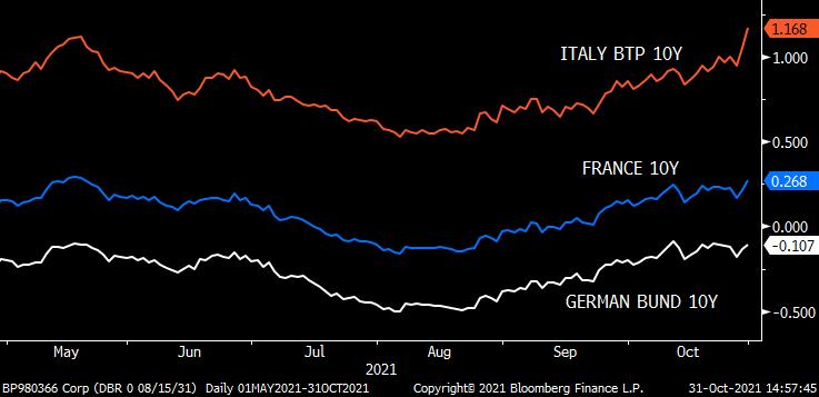
Source: Bloomberg

Inflation

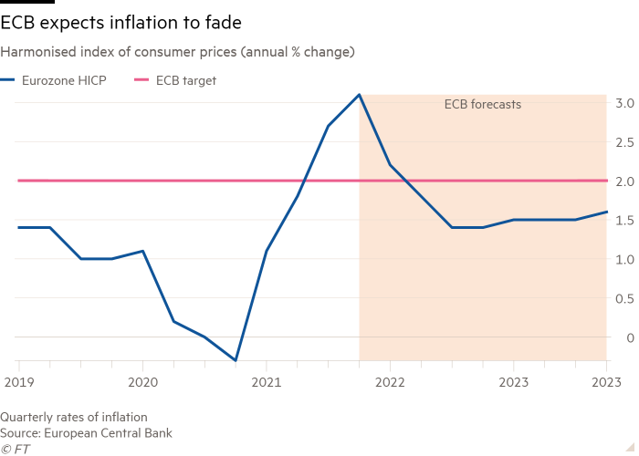
Source: FT

The ECB has long insisted that the current spike in prices is transitory and that underlying inflation pressures are unlikely to support future inflation levels to meet ECB targets. Currently, the ECB forecasts inflation at 2.2% in 2021, 1.7% in 2022 and 1.5% in 2023, thus below its 2% target.

In September, the HICP (official measure of inflation in Europe) skyrocketed to new historical highs since the GFC, while YoY PPI (Purchaser Price Index) Indexes are gaining ground at unprecedented speed: +14.2% in Germany, +13.3%, +13.4% in the Eurozone.

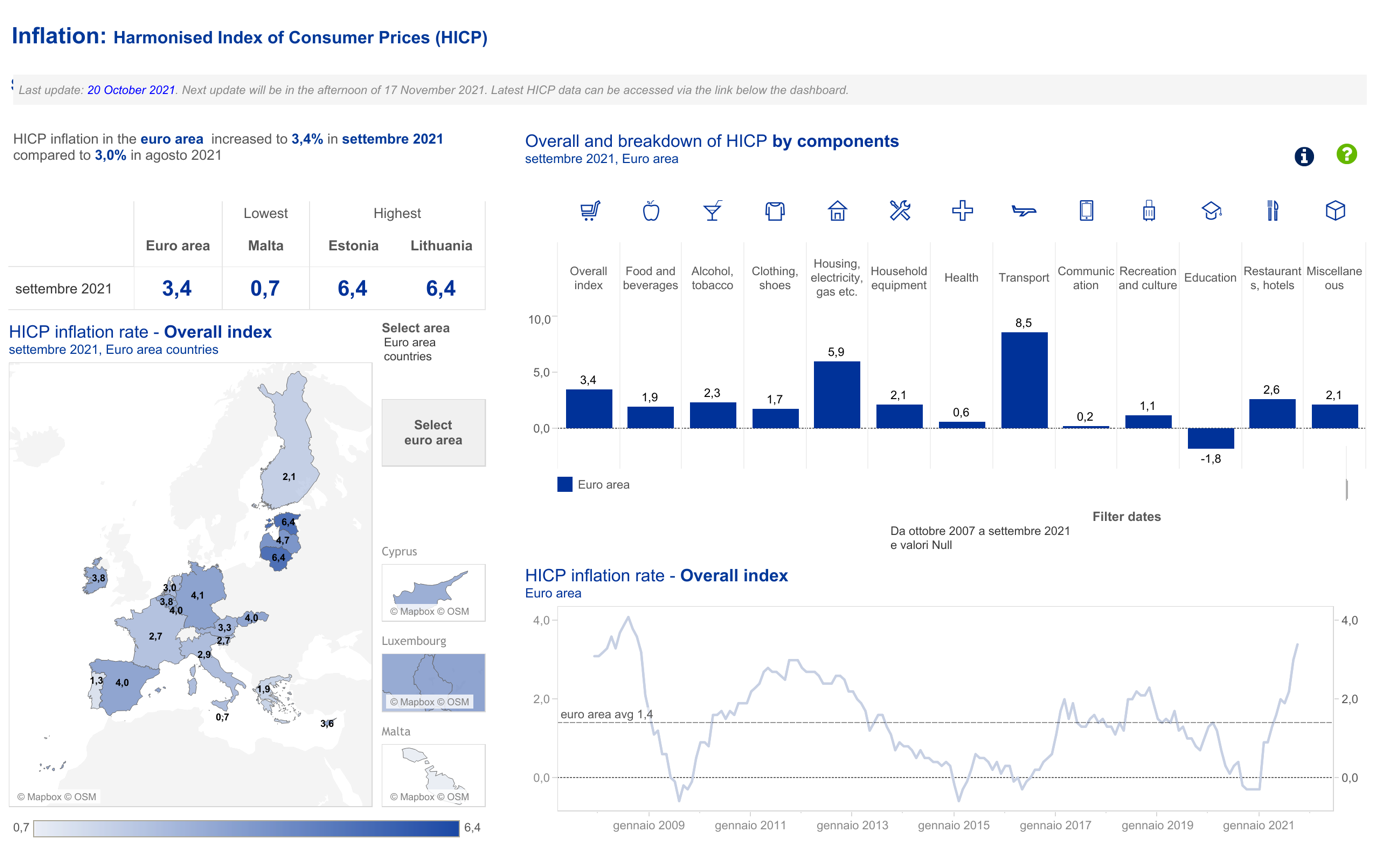
Source: ECB

Historically, Oil, gas prices movements are seasonal, characterized by downturns during summer and surges during winter. The recent price rush is determined both by insufficient supply – i.e., U.S. crude prices settled higher on Friday, turning positive after an early decline, supported by expectations that OPEC+ would maintain production cuts – and by upcoming winter seasons. We believe that the energy component will keep heavily impacting the overall index at least through Q1 2022.

Moreover, surging PPI is creating deep concerns on whether supply chain disruptions consequences will further increase prices charged to consumers, hence, it is fundamental to monitor consumer confidence for the following months and throughout the entire 2022 closely.

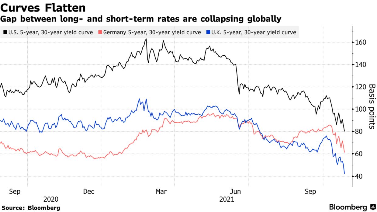
The big challenge for policymakers is the prospect of “stagflation” because of the recent rising inflation pressure and moderate consumer confidence. These fears are being reflected in the bond market in the shape of flattening curves where shorter-dated bond yields are rising much quicker than longer-dated ones.

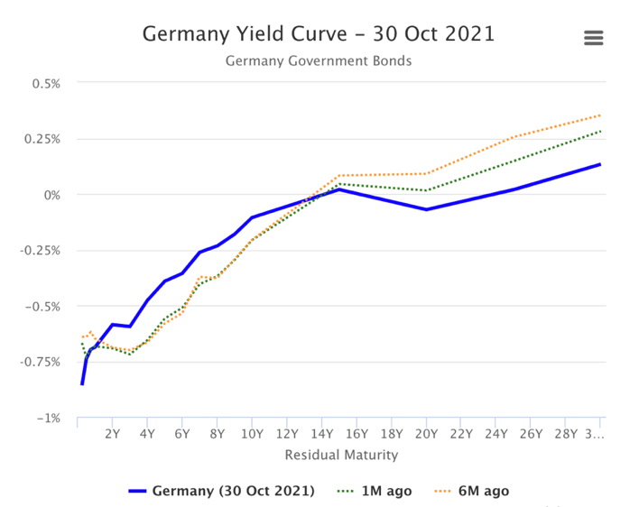
Source: Worldgovernmentbonds

The spread between Germany’s 2-year and 10-year bond and Germany’s 10-year and 30-year bond yields are at their narrowest since March 2020 respectively at 48 bps and 24 bps.

The narrowing spread between short and long-term yield, fuelled by central banks removing accommodative policies, gained momentum this week. The moves come as traders across global markets have been ratcheting up the outlook for policy tightening. The shift may have been reinforced after Brazil’s biggest interest rate increase in almost two decades and European bond market makers believing that rate hikes will come at the end of 2022.

Source: Bloomberg

The economic growth outlook continues to be uncertain and heavily dependent on the evolution of the pandemic. Currently, it is not clear whether rate hikes will be carried out at the end of 2022 or the beginning of 2023, and today’s low consumer confidence and rising energy prices are raising fears for lower future economic growth, all these factors have impacted the price of long term securities positively and that of short term bonds negatively. As the current macroeconomic forces will persist throughout 2022, we believe that it will result in the bond yield curve’s flattening.

We propose entering a 5y Bund long position and 30y Bund long position as an alternative to purchasing a bullet in the 10y Bund. In particular, the barbell portfolio would be constructed to cost the same and have the same duration as the bullet investment. The advantages and disadvantages of this barbell relative to this bullet will be discussed after deriving the composition of the barbell portfolio.

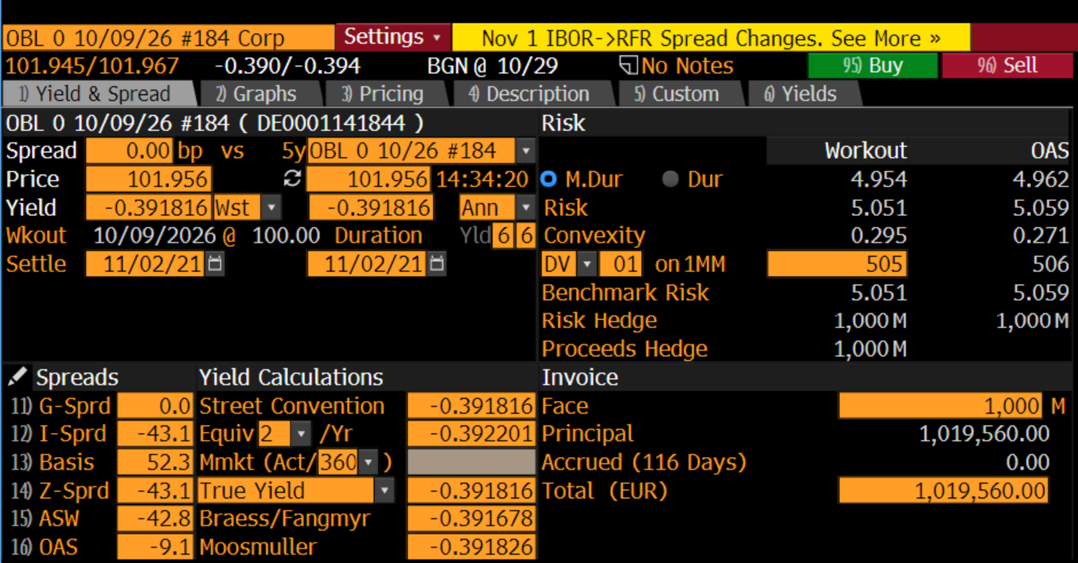
5-year Bund

10-year Bund

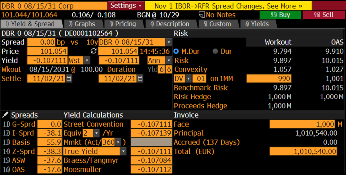
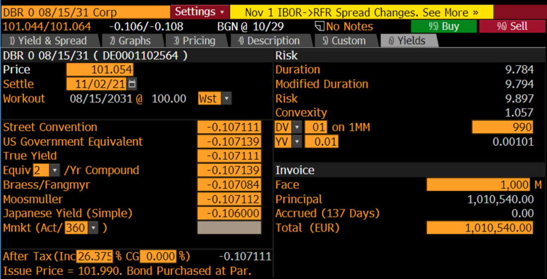
30-year Bund

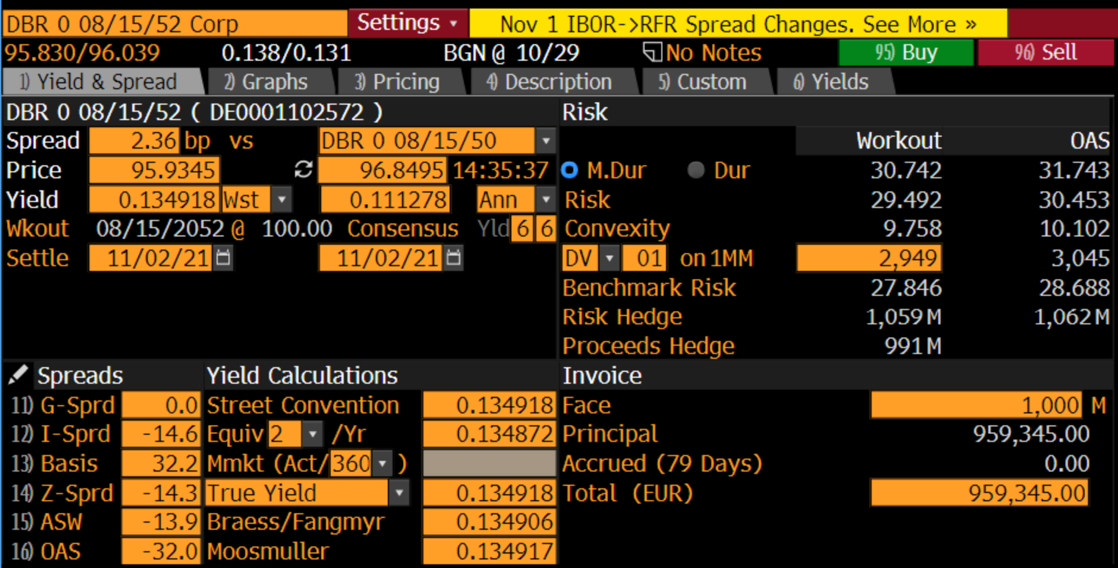
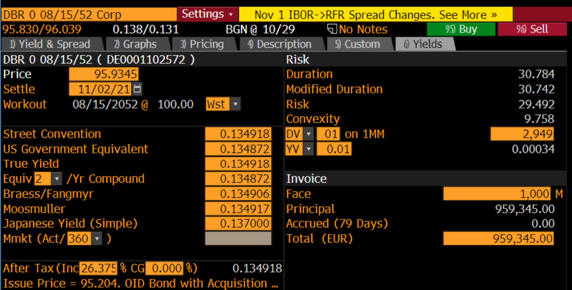
Source: Bloomberg

Let , and be the value in the portfolio of the 5y, 10y and 30y bonds, respectively. Then, for the barbell to have the same value as the bullet:

Furthermore, using the data from Bloomberg, we can compute the duration and the convexity of the equal weighted barbell portfolio:

The barbell (5.03) has greater convexity than the bullet (1.06). Return now to the decision of the portfolio manager. For the same amount of duration risk, the barbell portfolio has greater convexity, which means that its value will increase (decrease) more than the value of the bullet when rates fall (rise). On the other hand, the disadvantage of the barbell portfolio is its slightly lower yield:

compared with the yield of the bullet of -0.107%. Hence, the barbell will not do as well as the bullet portfolio if yields remain at current levels while, as just argued, the barbell will outperform if rates move sufficiently higher or lower.

Recalling the equations introduced in the previous paragraphs and assuming that the 5y Bund price will depreciate by 10%, while the 30y Bund will appreciate by 12%. We calculate the necessary yield change:

The necessary yield change for the 5y Bund and 30y Bund are respectively: 16.81 and 3.15. Both are definitely plausible, if we look at the basis-point movements in world bonds in the past few weeks.

References

[1] B. Tuckman, A. Serrat, Fixed income securities, Third edition