We gave a brief introduction to put writing strategies already earlier this semester. We since thought about possible modifications of such strategies and their effects on return characteristics and return predictability. The positive returns of put writing strategies can be motivated from risk premia, as we show in the first part of the article. We then investigate how the implied volatility surface is descriptive in explaining the returns of strategies that systematically sell put options of different maturities and strike prices. In the last part of the article, we recommend basing the decision of which option contract to short (by strike level and maturity) on the return neutralized from the underlying exposure.
Why put writing strategies generate positive returns?
We can break down a put writing strategy into two positions: lending at the risk-free rate and selling puts. Systematically selling puts generates positive returns. The economic intuition is simple: expected returns do not depend much on the investment’s volatility but rather on the correlation of losses with bad times in the market. As a result, investors demand high risk premia for investment strategies that perform poorly in bad times, when most risky assets underperform. Risk premia are particularly high for systematically selling puts because this is a strategy with a payoff characterized by steady small gains (collecting the option premium during bull markets) and by infrequent large losses (during bear markets). Just think of the simple CAPM model for expected returns; the asset volatility does not explain returns, while the beta does, which reflects the correlation with the returns of the broad investment universe. It is clear that systematically selling puts has the unappealing characteristic of a low beta when the market performs well (as we are selling puts we do not participate in the equity market upside) and a high positive beta when the market performs badly (as we are selling puts, we are hurt during market selloffs). This intuition is fully consistent with the empirical results that we found by running two regressions. In the former, we regress the excess return of the CBOE’s S&P500 PutWrite Index against the S&P500 excess return. In the latter, we regress the excess return of the S&P500 PutWrite Index against two factors: the excess return of the S&P500 when the return of the S&P500 is positive and the excess return of the S&P500 when the return of the S&P500 is negative. The second regression allows us to capture the non-linearity of the payoff of a put writing strategy. As we can see from the second regression output, the put writing strategy has a much higher beta when the market performs badly compared to when the market performs well (0.77 vs 0.42).


Monthly returns over the period September 2002-October 2019. Source of raw data: Bloomberg
Another theoretical explanation of why systematically selling puts is a positive return strategy can be found by using the framework of stochastic volatility models. In these models, there are two sources of risk in the market: the price of the underlying  and
and  its variance.

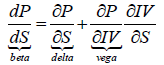
We describe their evolutions by using the Heston model. Notice that the model specification is not particularly important for our propose as we just look for an intuition of why systematically selling puts yields a positive return. Any model with stochastic volatility would provide this intuition. The expected excess return of any security/portfolio V will then be:

Where  and
and  are respectively the market price of equity risk and volatility risk, while and are the exposures to equity and volatility risk. The market price for equity risk is positive while the market price for volatility risk is negative because volatility is negatively correlated with equities so that it acts as a natural hedge (i.e. volatility is a negative beta asset) and so it deserves a negative market price for risk. By systematically selling puts we have a positive exposure to equities (we have positive delta) and a negative exposure to volatility (we have negative vega). By taking this into account, we understand why systematically selling puts has a positive excess return.
Can we predict put writing strategy returns?
We will now focus on finding some factors that can predict returns of put writing strategies. In this analysis, we will limit ourselves to put writing strategies on the S&P500. In researching potential predictors, we start from the basics of put options:
- The price of the option represents the cost incurred by the option buyer to insure against a selloff and the premium charged by the option seller for taking the opposite side of the trade.
- Implied volatility is the key determinant of the option price because it is the only non-trivial input of the Black and Scholes formula.
From this perspective, it seems reasonable that implied volatility could be a factor explaining put writing strategy returns. In fact, when implied volatility is high, we are selling expensive insurance, while when implied volatility is low we are selling cheap insurance. Therefore, we expect high implied volatility to predict high returns of the put writing strategy and vice versa.
Focusing only on implied volatility may be misleading. In fact, there may be good reasons why implied volatility is high, such as a highly volatile market where realized volatility is high. Therefore, with the perspective of a gamma trader, we want to sell volatility (short options) when implied volatility is high compared to realized volatility and so we will use the difference between implied volatility and realized volatility as a new predictor of put writing strategy returns. We use three methods to calculate realized volatility for the S&P500:
- Rolling window standard deviation of returns. This method has many well-known problems but it is straightforward to implement.
- Exponential weighted moving average. With this method, we compute volatility as a weighted average of the past squared returns, where the weights decrease exponentially. The exponential smoothing is a simple but effective technique to capture the typical volatility clusters. The smoothing coefficient is set at 0.95, which is a widely popular value among academicians and practitioners.
- GARCH. This method is widely popular in academia because it is a parsimonious model that captures many stylized facts about volatility. However, it is the most complex to implement as we first need to specify and estimate a model for the conditional mean. From the time series of realized returns and the time series of the mean returns derived from the model for the conditional mean, we obtain the residuals, which are then modelled using GARCH. As a first step, we specify a model for the conditional mean, choosing the ARMA models that maximizes information criteria. The model selected with this procedure is a moving average with 2 lags. This specification makes sense from an economic standpoint because there is no auto-regressive component, which would point at a market inefficiency because it would mean that one could predict S&P500 returns by looking at its returns in previous periods. On the other hand, a moving average process characterizes a partially efficient market in which news (i.e. the residuals) is incorporated with some delay. In our case of an MA(2) process, it takes 2 days to fully incorporate the news in market prices. Notice that the model was built using daily returns. Given the residuals, we estimate a GARCH(1,1) model and obtain realized volatility as output. Estimating a single GARCH model on the full sample of data would suffer from hindsight. In order to remove this bias, we estimate the conditional mean model and the GARCH model every month. Given the parameters estimated, we compute the return volatility throughout the month. On the next month, we re-estimate the conditional mean model and the GARCH model and use these parameters to compute the return volatility in the month. We iterate this procedure to cover the full sample.
It is worth recalling that realized volatility estimates are subject to the choice of some parameters such as the length of the rolling window, the smoothing parameter, the number of lags in the model for the conditional mean and the lags in the GARCH model. However, tilting these parameters does not materially change the results.
Finally, we considered as a potential predictor of put writing strategy returns the slope of the implied volatility skew. The slope of the skew represents investors’ expectations regarding the future skew of the return distribution: the steeper the implied volatility skew, the higher the probability assigned by the options markets to an extreme negative event over the tenor of the contract. Under Black and Scholes assumption of normally distributed returns, the implied volatility skew should be flat but, in practice, the skew is downward sloping in equities because investors expect the future distribution of equity returns to be negatively skewed. As we sell puts, we are exposed to extreme negative events and so the information content of the skew could be a valuable predictor. We compute the skew slope as the difference between the implied volatility of symmetric strike prices: 80-120% moneyness, 90-110% moneyness and 95-105% moneyness.
In order to test for predictability, we regress the 1, 3 and 6-month excess returns of the CBOE’s S&P500 PutWrite Index against each of the three factors (implied volatility, implied volatility minus realized volatility and the skew slope.). Results are summarized in the table below.
 Regressions based on the excess returns of the CBOE’s S&P500 PutWrite Index (PUT) over the period September 2002-October 2019.
Source of raw data: Bloomberg
The results of the regression show that the skew slope has no predictive power as regression coefficients are not statistically significant. We reported regression results only for the skew measured with 95-105% moneyness as it is the best performing (but still disappointing) among the other skew measure. Implied volatility does not explain 1-month returns, it is a statistically significant predictor for 3-month and especially for 6-month returns. As expected, the sign of the coefficient for implied volatility is positive which is consistent with the economic intuition that it is better to sell options when implied volatility is high. Notice that these results are based on a sample including the global financial crisis and so include for periods of rising volatility and sharp selloffs. The best predictor of S&P500 PutWrite Index returns is the difference between implied and realized volatility, with statistically significant coefficients and decent R-squared. The sign of the coefficient is positive which is consistent with the economic intuition that it is better to sell options when implied volatility is rich with respect to realized volatility. Notice that the results reported in the table refer to realized volatility as measured with GARCH, while realized volatility as measured by exponential weighted moving average and standard deviation do not lead to predictability.
Better predictability for different moneyness?
The S&P500 PutWrite Index is only one of the possible put writing strategies, specifically one built by shorting at-the-money puts with one month and three months to maturity, respectively. In this section, we will abandon the CBOE index and build our own put writing strategy. This will give us more control over the moneyness of the options and their tenor, and so will allow us to explore the predictability of put writing strategies returns beyond those strategies built with at-the-money options. Moreover, we are able to reconstruct the returns of these strategies since January 1996, so that we have a larger sample covering two recessions (2001 and 2008). We focus on put writing strategies built by shorting out-of-the-money puts. These strategies have lower exposure to the stock market (out-of-the-money options have a lower delta in absolute value) and so will be hurt less by market selloffs. We arbitrarily choose to focus on put options with 90% moneyness, defined as strike price divided by the forward price. We built two put writing strategies on the S&P500 that every month short puts with 90% moneyness and invest the present value of the option’s strike price at the 1-month US Libor.

Notice that, for put-call parity, this strategy should be equivalent to a covered call strategy in which we are invested in the underlying (S&P500) and short calls. We roll our position on the third Friday of every month (this is the same roll technique employed by the CBOE when building the returns of the S&P500 PutWrite Index). The two put writing strategies that we built differ on the tenor of the options shorted:
- 30-day strategy: the strategy is built by selecting at each roll date the options with a 90% moneyness and maturity as close as possible to 1 month. On each roll date, we buyback the option shorted if it has not expired yet. If it has expired, we simply pay its payoff.
- 90-day strategy: the strategy is built by selecting at each roll date the options with a 90% moneyness and maturity as close as possible to 3 months. In some cases, the options with maturity as close as possible to 3 months were options with maturity as low as 2 months and as high as 5 months. Nevertheless, the average and median maturity of the option selected is 90 days. On each roll date, we buyback the option shorted at the prevailing market price.
In the following charts, we plot the cumulative return and the excess return of the two strategies. As expected, the lower delta of the strategy shorting 1-month puts results in less volatile returns and less exposure to left tail events than the strategy shorting 3-month puts. Moreover, the strategy selling longer-term options generates more yield enhancement (and so higher returns) because longer-term options have a higher premium. Over the timespan ranging from January 1996 to May 2019, the 3-month put writing strategy has an annual mean excess return of 3.78% and an annualized volatility of 5.59%, while the 1-month put writing strategy has an annual mean excess return of 2.65% and an annualized volatility of 4.34%.


Source of raw data: Wharton Research Data Services, OptionMetrics
From the chart plotting the excess return of the two strategies, we get a clear idea of the behavior of a put writing strategy which has a capped upside (as we are selling puts we do not participate in the equity market rise) and full downside participation (as we are selling puts, we are hurt during market selloffs).
We then regress the 1, 3 and 6-month excess returns of the two put writing strategies against implied volatility and the difference between implied and realized volatility. Implied volatility is measured by VIX. We omit results referring to the slope skew since it has no predictive power.


Regressions based on the excess returns of the two put writing strategies over the period January 1996-May 2019. Source of raw data: Wharton Research Data Services, OptionMetrics
The regression results reported in the tables show that both implied volatility and the difference between implied and realized volatility are statistically significant predictors of put writing strategy returns. In particular, implied volatility is a good predictor 3 and 6-month returns of put writing strategies on out-of-the-money options. Notice that R-squared is much higher for put writing strategies on out-of-the-money options than that for the CBOE put writing strategy on at-the-money options.
How the implied volatility surface can be used to estimate the volatility risk premium embedded in option contracts
As stated at the beginning of the article already, the pricing of options requires to make assumptions on the dynamics of the underlying’s price and variance rate. The most popular of such models is the Black-Merton-Scholes (BMS) model. It’s far from a well-kept secret that the BMS model assumptions are violated. Thus, institutional investors don’t express their views on volatility in quoting option prices, but through the implied volatility in option prices derived from the BMS model. The BMS model is thus used to transform the information embedded in option quotes and to derive the implied volatility surface. The convention of quoting implied volatility further seems to be attractive as it directly excludes arbitrage between the option and its underlying asset. This highlights the reliance of market practitioners on the implied volatility surface. But per se, the implied volatility surface is a price surface. Trying to get information about the profitability of selling options would be similar to estimate the return of buying a stock based simply on its price. Carr and Wu (2016) propose a new modelling framework to model the implied volatility dynamics and derive direct implications on the shape of the implied volatility surface. They impose a simple algebraic constraint on the shape of the prevailing implied volatility surface by transforming the dynamic, no-arbitrage constraint between the underlying stock, a basis option and any other option. This allows them to estimate the difference between expected and implied volatility for each option contract. They find that implied volatility is typically higher than expected volatility, thus documenting a volatility risk premium. However, they also find that the option surface is affected by more than the underlying’s assets dynamics. Their presented framework of option-specific realized and expected volatility opens a new opportunity for option-specific volatility forecasting.
One should be aware though that the relationship between the volatility risk premium and the returns of option selling strategies is imperfect: options experience time-varying exposure due to their path-dependency. Thus, for investors who want to benefit from the volatility risk premium, it would make sense to take a closer look to the properties of the returns generated from selling options than to focus solely on the difference between implied and realized volatility, on which we elaborate a bit further in the sect paragraph.
What are alternative measures to identify the “richness” of option contracts
To analyze the attractiveness of the returns generated by a short position in put options, it would be more appropriate to look at the returns attained that are not due to the equity exposure inherent in such a position. The logic behind such thinking is that one would not need to sell option contracts to obtain the equity risk premia of the index. This can be done much simpler (and less costly) by a long position in an ETF. The framework presented builds on Israelov and Tummala (2017). The simplest way to hedge against price changes in the underlying is known as delta hedging. This is most commonly done by hedging the Black-Scholes delta exposure,

which describes the excess returns generated by the put writing strategy, after delta hedging by means of a position in S&P 500 index futures equivalent to the delta coefficient. The last term in the numerator accounts for the interest earned on the option’s premium. If one would analyze option returns on such measure, shorter-dated options show higher average returns than longer-dated ones. Similarly, deep out-of-the-money (OTM) option contracts show lower returns than option contracts closer to at-the-money (ATM). This can be explained by the lower volatility exposure of OTM options. Therefore, to have a level playing field in terms of evaluating the “attractiveness” of option contracts, one also needs to consider their exposure to changes in implied volatility. Hull and White (2015) show that this can be measured by beta which they define as,
The implied volatility of an option contract changes according to market dynamics. If the equity index drops, implied volatility rises, whereas in a bull market it usually declines. We, therefore, would expect delta-hedged short positions in put options to have a positive beta, thus generating losses when implied volatility increases. As mentioned before, ATM and longer-dated options are expected to have higher beta values due to their higher exposure to implied volatility. When evaluating the excess returns of options strategies, it would, therefore, be more appropriate to neutralize the returns by the above-described equity exposures, since such defines the performance of short positions in option contracts that can’t be obtained elsewhere.
The effects of changing strike levels and maturity of short puts
By analyzing the performance of put writing strategies on the S&P 500 index we considered strategies that varied in the maturity and strike level of the sold option contracts. For shorter-dated options, two offsetting effects hold true: they have a higher gamma exposure than longer-dated options, while at the same time having a smaller vega exposure than their longer-dated counterparts. Complicating this is the fact that short-dated implied volatilities tend to change more than longer-dated implied volatilities. Israelov and Tummala (2017) find that the higher gamma exposure is more impactful than the lower vega exposure for options with one month to maturity.
Another interesting finding of the two researchers concerns the risk-adjusted performance between OTM and near ATM put writing strategies. While OTM options are better compensated on a risk-adjusted base when evaluating risk in terms of return volatility, this doesn’t hold true when looking at the performance of the two strategies under stressed conditions (e.g. an index drop of 20%). Under such conditions, near ATM short option strategies seem to be better compensated which the authors argue with the higher demand of investors for put options with strike levels just below the prevailing spot. Investors thus need to decide which risk metric to use when evaluating the attractiveness of the compensation for the risk of options with different strike levels.
Conclusion
In order to assess the richness of option contracts, we tried to obtain information from the implied volatility surface. While this approach seems to work much better for the return series of selling OTM options, there was only very limited descriptive power for returns of shorts in ATM put options. However, we found that the opposite relationship holds true for the difference between implied volatility, measured by the VIX index, and realized volatility, measured with a GARCH(1,1) model. Returns of short positions in OTM longer-dated options seem to be better described by changes in implied volatility than the return series of shorts in their shorter-dated counterparts. Even though put-writing strategies expose the investor to tail events, the skew in the implied volatility surface, measured as the difference in the implied volatility of 80-120%, 90-110% and 95-105% moneyness options, didn’t contain any information content of the returns from selling options, regardless of maturity or strike level. Such limited relationship between the returns of selling options and the risk premia paid for volatility further stresses the importance of assessing the attractiveness of options with different maturities and strike levels not solely based on the volatility risk premia but on other the isolated return characteristics of the option-selling strategy, as highlighted towards the end of the article.


0 Comments