Dislocations Between Historical and Implied Volatility as an Indicators of Volatility Trades

Differences between historical realized volatility and option implied volatility has for long been known as a potential indicator for volatility mispricing. To our knowledge, the first well-known academic study on the topic was conducted by Goyal and Saretto in 2009 and published as the paper ‘Cross-section of Option Returns and Volatility’. We will first start with a brief explanation of the contents of the paper and the broad idea. We shall then proceed to conduct a preliminary investigation on whether the indicator could potentially work.

Overview of Goyal and Saretto, 2009

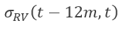
The authors sort a universe of stocks on the basis of the difference between the realized historical volatility over the last 12-months (12m HV) and 1-month options implied volatility (1m IV).

The authors then sort stocks in descending order of their indicator value in each month. They then study the results of 2 different strategies:

1. Long (short) straddles of highest (lowest) deciles based on the indicator
2. Long (short) delta hedged calls of highest (lowest) deciles based on the indicator

Since the indicator varies based on the time-point in which it is computed , the portfolios’ stocks must be changed every month.

The basic thesis is that volatility mean reverts and, therefore, 1m IV should reflect the fact that future volatility will, on average, be closer to its long-run average historical volatility (12m HV) than to its current volatility (HV for periods lesser than 12m). If this were to be true, a large value of indicator would mean 1m IV is under-priced and vice versa.

The authors find statistically significant returns on both the long vol and short vol legs of the trades even after accounting for transaction costs and larger margin requirements for the short legs. For example, a long-short decile portfolio of straddles yields a monthly average return of 3.9% (MoM)after considering transaction costs.

To further understand the underlying reasons of the empirical regularity, the authors study the behaviour of volatility (IV and HV) around the portfolio formation date.

They find that the deviations between HV and IV are transitory—on average, there is very little difference between the two volatility measures one year before and after the portfolio formation , while at the portfolio formation month, by construction, has large deviations between 1m IV and 12m HV.

Research shows that stocks with a large positive indicator , at a certain portfolio formation date, show significantly positive returns in the month just preceding this date, and the stocks with a large negative indicator have significantly negative returns in the month just preceding. The fact that temporary deviations of IV from HV are preceded by extreme patterns in stock returns suggests that investors overreact to current events, increasing (decreasing) their estimate of future volatility after large negative (positive) stock returns.

Analytical Derivation of the Indicator

Before jumping on analysing the behaviour, we derive an interesting result.

1. By looking at the Black-Scholes partial differential equation, and assuming 0 interest rate (which can be practically implemented by replacing the underlying with its Futures when options and futures have expiration on the same date)
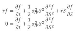
2. Recall the break-down of options’ Greeks

where:

• Delta (δ) : sensitivity of the option price to changes in the underlying
• Gamma (Γ) : sensitivity of the option delta to changes in the underlying (i.e. derivative of )
• Theta (θ): sensitivity of the option price to changes in passage of time
• Vega (V): sensitivity of the option price to changes in implied volatility
• Others: changes in interest rates, dividend expectations, and higher sensitivities (ex. 3^rd derivatives)

Fortunately, it is quite easy (but somewhat expensive) to hedge the delta, we can do this by entering in an offsetting position on the underlying in the quantity specified by : practice known as delta-hedging.

3. Finally, by performing:

• Delta hedging
• Neglect the “others”

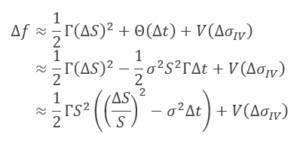
This results shows that the daily change in option price depends (approximately) on the summation of:

1. Gamma + Theta PnL
   • Difference between one-day realised variance (proxied by one-day return squared), and one-day implied variance multiplied by the dollar Gamma (1/2ΓS²)
2. Vega PnL

Point a resembles the indicator that Goyal and Saretto have been looking at, in fact, by assuming a constant Gamma over 1m, and constant volatility, the term in brackets is the difference between ex-post realised and ex-ante implied volatility.

Our Preliminary Investigation into the Viability of this Indicator

Doing a full-fledged back-test at this stage would be data intensive and time consuming. We would need to construct delta hedge straddles (at least 2-3 straddles on each stock to keep Vega and Gamma alive as the spot moves around during the life of the trade) on many stocks, each month, and over around 10 years.

So, we decided to first study the behaviour of the volatility of the stocks with the highest absolute values of the indicator. If their behaviour is proved to be as expected, then we could potentially conduct back-test using straddles.

Before we delve into the specific of what we studied, it would be useful to get some terminology out of the way.

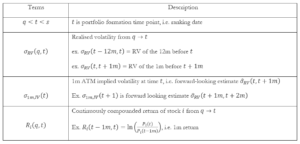
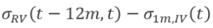
We start with all the S&P 500 stocks. Then, for each month from 2006 to March 2017, we calculate the trailing 12m RV of each stock, take the ATM 1m IV and calculate the indicator:

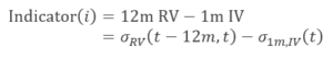
We then rank the stocks in descending order based on their indicator’s value and take:

1. Basket of top 20 stocks, which we call “Long vol basket”
2. Basket of bottom 20 stocks, which we call “Short vol basket”

For each (monthly) time point over the 11years, the stocks composing each portfolio will be changing over time.

Overall, we study the following things

1. We break up the hypothetical delta hedged straddle returns into 2 Indicators
2. A Gamma + Theta P&L indicator – the sign of our indicator  will determine the sign of our Dollar Gamma P&L 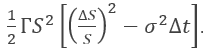Ideally, we would expect this to be positive for the long vol basket and negative for the short vol basket.
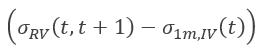
3. A Vega P&L indicator – we study the change in ATM 1m IV as a proxy for this. In other words, we study the sign of 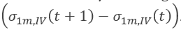Ideally, for the long basket, this should be positive and for the short basket, negative.

Note that we are taking a slight shortcut here. We should, theoretically, study the change in IV of options of the same tenor (If we go long a 1month option, we should study change in its IV as the maturity falls to less than 1 month). However, we are using 1m ATM IV as a proxy for this. This seems to be conceptually sound – if 1m ATM IV increases, it’s likely it was underpriced before and vice versa.

Please note that we refer to the two points above as Dollar Gamma and Vega P&L Indicators. Practically, both Vega and Gamma P&L’s are path dependant as our Gamma and Vega change and the final P&L depends on our daily exposures to the two risk factors. For instance, we might have unfavourable Dollar Gamma P&L despite the Dollar Gamma Indicator being favourable because the Gamma exposure isn’t managed properly.

1. We study what causes the deviation in between  and  using the following

• Preceding month return, or
• Difference between 12m HV and 1m HV preceding the ranking

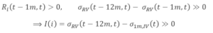
Ideally, the long vol basket should have a significant positive preceding month return and positive difference in 12m HV and 1m HV preceding the ranking

The stock experienced one month of significant positive return, leading to a small monthly realised volatility , this is driven by the stylised fact that positive returns are usually small and negative returns big – the market overreacted and expects and even smaller vol for the next month, implied by a small Results

By taking a double arithmetic average over each basket’s stocks and over the 11y, i.e. average of the panel of data. We obtain the following results:

Long basket:

1. Initial Dislocation: 16.63%
2. Gamma and Theta P&L Indicator: -0.40%
3. Vega P&L Indicator: 4.08%

: 12.33%

5. Preceding month return: 2.99%

Some takeaways –

• The preceding month return is significantly positive and so is This explains the large indicator 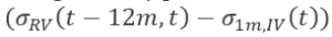In other words, the low 1m ATM IV at the date of ranking seems to be driven by a fall in the 1m RV preceding the day of ranking, which in turn, seems to be driven by a significant positive return.
• The Vega P&L Indicator is positive – The 1m ATM IV seems to increase consistently following the day of ranking – this is good news.
• The Gamma and Theta P&L Indicator is negative – the loss from Theta would marginally dominate what we make from Gamma. While this is not great news, the good news is that the 1m ATM IV change is significantly larger.

Short basket:

1. Initial Dislocation: -14.77%
2. Dollar Gamma P&L Indicator: -5.79%
3. Vega P&L Indicator: -6.58%

: -4.83%

5.Preceding month return: -2.15%

Some takeaways –

• The preceding month return is significantly negative and so is This explains the large negative In other words, the high 1m ATM IV at the date of ranking seems to be driven by a rise in the 1m HV preceding the day of ranking, which in turn, seems to be driven by a significant negative return.
• The Vega P&L Indicator is negative – The 1m ATM IV seems to decrease consistently following the day of ranking – this is good news since this is a short vol basket.
• The Gamma P&L Indicator is negative – This is good news. Also, notice how this is significantly negative for the short vol basket (but only marginally negative for the long vol basket). This makes sense because we’re monetizing the volatility risk premium when we short options as well as benefiting from time decay – while both these factors hurt us for the long vol basket.

Overall, we think that this is worth a full-fledged back-test to see the results when we carefully manage our Greeks.

We can obtain quite a few takeaways from this brief analysis:

1. Even if this doesn’t make sense as a stand-alone systematic strategy, our results show that  can be used as a factor to predict the change in 1m ATM vol, and judge the cheapness or dearness of volatility baked into option prices
2. The general idea that implied volatilities always overestimate in the upside the realised volatility is untrue: market overreacts to returns by estimating IV both higher and lower than RV based on the most recent return, i.e. the market, in general, is momentum-following in the short term.
3. Overreactions in IVs tend to ease in the following months and reverting to their long-term RV
4. Another empirical proof that following positive returns, volatility falls. While following significant negative returns, volatility rises

Download as PDF