Fixed Income Trading: Unlocking Risk Reduction with OLS and PCA Hedging

Download PDF

Introduction

In fixed income trading, managing interest rate risk is a critical task for traders and portfolio managers. While traditional hedging tools that rely on duration or convexity are a good indication of how prices react to yield changes, they are based on limited assumptions with significant pitfalls in practice, leaving portfolios vulnerable to a lot of undesired risks.

As a response to these shortcomings, more sophisticated approaches like Ordinary Least Squares (OLS) regression and Principal Component Analysis (PCA) hedging have gained attention. These methods offer a deeper analysis of interest rate movements by considering multiple factors or components, providing a more precise way to capture the complexities of yield curve changes. This article delves into the limitations of traditional hedging methods and introduces OLS and PCA as alternatives for more effective risk management.

Through this discussion, we’ll explore how OLS and PCA can be applied to real-world scenarios, by presenting a trade idea and demonstrating how these methods can generate more accurate hedging weightings. Our goal is to provide a comprehensive view of why these advanced techniques offer a more precise and robust hedging in today’s complex fixed income market.

Caveats of traditional Hedging

In the world of fixed income markets, interest rate risk is a crucial concept. It measures how much the price of a security changes when interest rates fluctuate. This inverse relationship between a bond’s price and yield means that investors and traders need to understand how sensitive a bond’s price is to changes in interest rates to be able to accurately plan their investments and anticipate outcomes. Knowing the interest rate risk also helps investors protect, or hedge, their investments by undertaking steps to reduce this risk.

There are two basic methods to measure interest rate risk: duration and convexity.

Duration measures how sensitive a bond’s price is to changes in interest rates. In this article, we will discuss two types of duration:

1. Modified Duration estimates the percentage change in a bond’s price for a 1% change in yield. For instance, if a bond has a modified duration of 5 years, a 1% increase in interest rates would result in a roughly 5% decrease in the bond’s price. It’s a useful measure for understanding how much a bond’s price could move with changes in interest rates, but it assumes a simple, linear relationship between price and rate changes. The formula to compute it, where YTM stands for yield to maturity, n represents the number of periods per year when coupon is received, and Macaulay Duration is the weighted average term to maturity of the cash flows from a bond:

1. DV01, which stands for ‘dollar value of 01’, is another measure of bond duration that tells us how much the price of a bond will change in dollar value if interest rates move by 0.01%, or 1 basis point. For example, if a bond’s DV01 is $50, it means that for every 0.01% increase in interest rates, the bond’s price would decrease by $50. It is a straightforward measure that is often used by traders to understand small, immediate changes in price. The formula to compute it, where stands for the change in market value of the bond and represents the change in yield, is:

Convexity builds on the idea of duration and adjusts for its limitations. While duration assumes that price changes are linear, convexity accounts for the fact that the relationship between a bond’s price and interest rates is actually curved, not straight. Bonds with high convexity tend to gain more value when interest rates fall and lose less value when rates rise, compared to bonds with low convexity. The formula to compute it is:

These measures are also known as one-factor formulations because they are usually based on the idea that interest rates across different maturities move in a coordinated way. In other words, they carry the assumption that rates for all maturities move up or down by the same amount, causing a parallel shift in the yield curve. Therefore, these models predict that when the rate of a bond with a certain maturity changes, the rates for other maturities adjust accordingly.

However, reality is unpredictable and cannot be fully portrayed by a simple linear or curved model. In fact, each of these methods has notable limitations that make them less effective in certain market conditions.

As already mentioned, for example, duration relies on a linear assumption. When interest rates move significantly, duration’s accuracy diminishes because it does not account for the curvature in the price-yield relationship. This limitation makes it a “local” measure – it accurately estimates price changes near the current rate but requires frequent modification as rates change, which can increase trading costs.

Convexity attempts to address this issue by considering the non-linearity of the price-yield relationship, offering a more accurate measure when rates change significantly. However, calculating convexity is more complex, requiring advanced models and tools, which can be a challenge for some investors. Additionally, both of these measures assume that interest rates across all maturities move in parallel – a scenario that, as mentioned, rarely occurs in practice. In reality, the yield curve often steepens or flattens, with short-term and long-term rates changing independently, and duration cannot account for these shifts.

Therefore, these limitations mean that, while duration, and convexity offer foundational insights into interest rate risk, they can be insufficient in capturing the full complexity of market movements, often necessitating the use of more sophisticated models as the ones discussed further in this article.

Trade Idea

In this section, we propose a trade idea that will serve as the basis of our OLS and PCA-based hedging applications, however we want to stress out that fundamental research is not the main scope of this article, so there might be better trades in the current environment. A 2Y-5Y-10Y butterfly trade is a bond trading strategy that focuses on changes in the shape of the yield curve, specifically its curvature. This trade involves shorting 2-year bonds, going long on 5-year bonds, and shorting 10-year bonds. The idea is to profit from a scenario where yields on 2-year and 10-year bonds rise more than the 5-year bond yield. In this setup, the trader is betting on a positive butterfly shift in the yield curve, where the “wings” (2-year and 10-year) rise faster than its “body” (5-year).

The main fundamental rationale of this trade is that, in our view, the market has priced in too much easing by the FED in the upcoming meetings. Currently, the Fed Funds Futures are pricing in 89.5% chance of a 25 basis points cut at the November meeting, and 84.5% of 50 basis points to be cut by the December meeting. While we still see the scenario of 2 cuts by year-end possible, we believe the probability for only one is overlooked, recently leading to a slight steepening of the 2Y-5Y part of the curve. With inflation declining very slowly at this stage, real growth still being way above implied by a disinflationary environment and a strong labor market report released recently, we believe that the FED needs more data to make a concrete decision of cutting twice as of now. We see a few catalysts that can keep inflation sticky in the short-term: supply disruptions caused by the hurricanes, falling immigration that could be an inflationary force (immigrants benefited the US labor market by providing high productivity at low costs) and rising oil prices caused by the war in the Middle East. As for the long-end of the curve, we think it is poised to stay higher than expected over the coming years, spurred by the significant fiscal deficit accumulated by the US. Moreover, both sets of policies proposed by the two presidential candidates are inflationary and seem to already have had an effect on the 10Y yields recently.

We foresee a trade horizon of 1 to 2 months, but we keep an eye on potential economic surprises that could endanger our position, in this case data prints/events that would price in more easing. In the following two sections, we will assume a notional of million for the 5Y leg and will calculate the and notionals of the other two legs, in accordance to the statistical tools proposed. We will also use the following estimates, according to the most recent Bloomberg data: = 186, = 442 and = 794.

Alternative 1: OLS-based Hedging

Ordinary Least Squares (OLS) regression is a useful hedging tool in fixed income markets for several reasons. The core idea is that OLS helps quantify and model the relationships between different interest rate instruments and other risk factors.

OLS regression can model the relationship between the yields of different fixed income assets. For example, you can use OLS to estimate how changes in the yield of a 10Y bond are related to changes in a 2Y bond or to the overall interest rate curve.

The model enables traders and portfolio managers to understand how sensitive a bond’s yield is to changes in other variables, which is essential for hedging interest rate risk.

OLS finds the slope of the regression, represented by beta, which is a gauge for the sensitivity of one asset to the other. For example, you can regress bond prices (or returns) on changes in interest rates to understand how a bond’s value will move in response to interest rate fluctuations.

This allows for a more optimal duration hedging, where the sensitivity of one asset to another is taken into account too, in addition to DV01 or other measures mentioned before. OLS can be applied to determine the optimal hedge ratio by regressing the returns of the bond or fixed income portfolio on the returns of the hedging instrument (e.g., futures or swaps). This is similar to how the beta coefficient in stock market hedging measures the sensitivity of an asset to market movements.

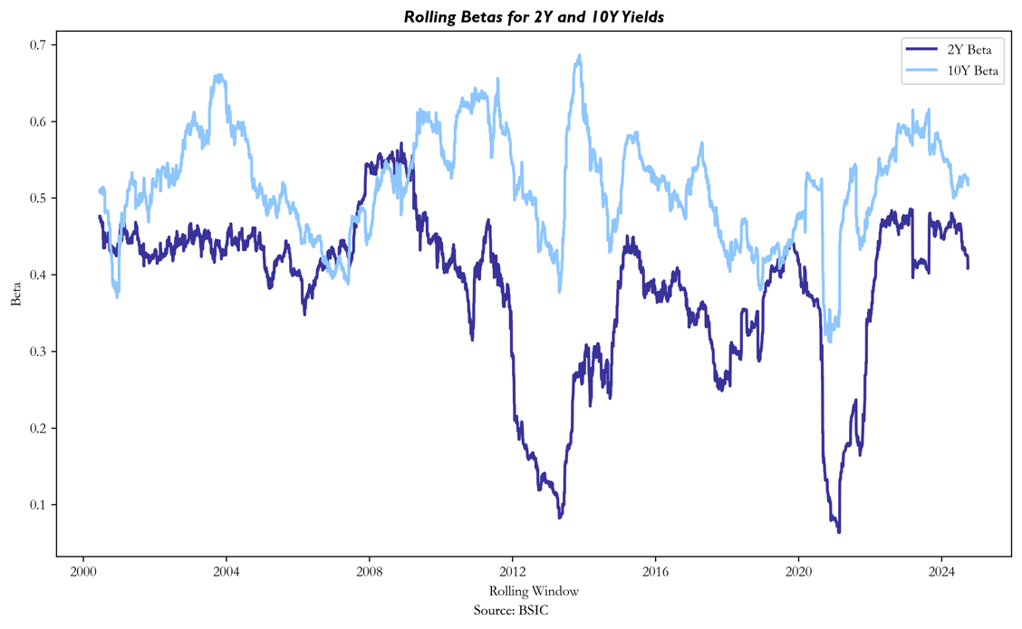
In financial analysis, asset relationships often evolve over time, making it critical to account for dynamic changes in market conditions. One effective way to capture this time-varying behaviour is through rolling Ordinary Least Squares regression. Unlike traditional OLS, which estimates a static relationship using the entire dataset, rolling OLS re-estimates the regression parameters over a moving window of fixed size. This allows us to track how the coefficients, such as beta or sensitivity to market factors, change as new data points are introduced and older ones are excluded.

This approach is particularly useful for understanding trends in financial markets where correlations between variables – like stock returns and macroeconomic factors – are not constant. By applying rolling OLS, we can assess how these relationships shift, offering deeper insights into risk management, portfolio optimization, and market dynamics.

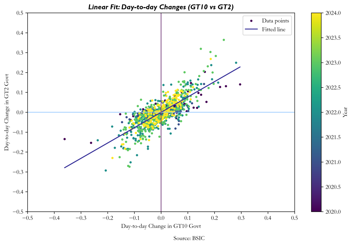
In our study, we applied a rolling OLS to analyse the evolving sensitivity of 5Y yields to 2Y and 10Y yields, in a multi-variable model. We downloaded mid-yield data of CMTs (Constant Maturity Treasuries) for the 2Y, 5Y and 10Y tenors that we are using in our trade, from the 3rd of January 2000 to the 1st of October 2024. By using a rolling window of 120 days, we were able to track how the sensitivity of bond yields to market factors varies over time.

In practice, regression-based hedging can closely align with simpler DV01-based hedging but introduces a small yet critical adjustment via the regression coefficient . This coefficient offers greater precision, allowing for more accurate adjustments to the hedge.

Accordingly, the formulae used to calculate the notional value of the other two legs simply incorporates the beta term in the durational-neutral hedging:

By solving the above equations using the latest betas estimates obtained, = 0.4103 and   = 0.5172, we obtain = -$97.51 million and = -$28.79 million. These amounts are to be shorted in 2Y and 10Y bonds respectively, for every $100 million bought in 5Y bonds.

Alternative 2: PCA-based Hedging

Another useful statistical tool to provide the adequate weightings for the legs of our trade is Principal Component Analysis (PCA).

PCA decomposes the market inputs into a set of uncorrelated and linear returns, describing the shape of the market mechanism, expressed by eigenvectors and how strong the relationships are relative to each other within the given market mechanism, expressed by eigenvalues.

Specifically for fixed income applications, PCA can provide an empirical description of the behaviour of the entire term structure that can be applied to any bond. In practice, it can use the bond yields or swap rates with maturities starting from 1 to 20 or 30 years as inputs and find the sensitivities of each tenor to the main principal components (PC), measured in basis points changes per one standard deviation of the respective component. This will help us later when deciding how much to hedge each leg. What’s more, the first three PCs, that usually explain at least 99% of the variance present in the variables of interest, link their mathematical form with an economic intuition. As will be interpreted later from the results, in the fixed income market, PC1 is associated to the “level” of rates, PC2 to the “slope” of rates and PC3 to the “curvature” of rates.

Model Implementation

We used the same data and time interval as for the OLS regression model. Our goal is to implement a rolling PCA with a rolling window of 120 days, as the two biggest pitfalls with using PCA are correlation between factors (supposed to be uncorrelated) in sub-periods and the instability of eigenvectors over time (change in market mechanics). The choice for the size of the rolling window reflects a stable trade-off between smoothing out short term noise and not capturing shifting market dynamics too late. Before running the PCA, some further transformation is required in order to obtain relevant results. Firstly, we need to demean the data, shifting the distribution to a zero mean so that the analysis focuses on the variance and covariance of the series. Also, in order to properly use PCA, the time series have to be stationary, so we used de-trending as a method to “stationarize” the level of yields.

Finally, we ran the PCA using only 2Y, 5Y and 10Y as defined by our trade, but as a general practice, data for all tenors can be used to generate other trade ideas or before deciding on the specific maturities of the trade.

A common issue that becomes apparent when running a PCA is the sign inversion of eigenvectors. Given any eigenvector which satisfies all constraints for PCA, the same eigenvector multiplied by -1 will also satisfy the problem. The “sign flipping” effect can happen to any principal component and each component is affected independently of another. When running PCA recursively, a switch in component signs from one period to the next time will result in the entire reduced data for that period being multiplied by -1 and will completely alter the output of the remaining data. To fix this, we used the cosine similarity score, that can be computed as the dot product of eigenvectors, given they are unit vectors. The similarity scores will recursively link principal components in sequential time periods and will un-flip the eigenvectors should the cosine similarity score be below 0.

Interpretation of Results

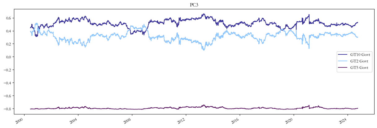
In the three charts below, you can see the factor loadings for each PC and tenor present in our analysis. A higher absolute value of the loadings indicates a stronger influence of that tenor on the respective PC, whereas its sign represents the direction of the influence. The results correspond to the standardized version of the change in yields, as this reflects a more accurate picture. When running the PCA on either the level of yields or on non-standardized data, we noticed some non-stationarity coming back into play even though we de-trended the data.

Moving on to the interpretation of the plots, we can notice that the loadings for PC1 are all positive and in a tight range, as PC1 is associated with the “level” component and the sensitivities of each tenor can slightly vary across different regimes.

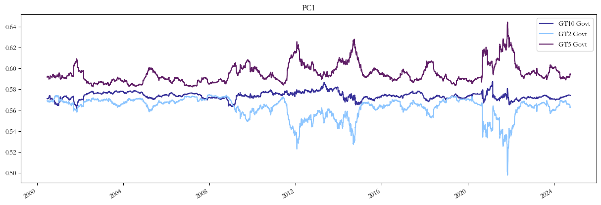
On another note, the loadings for the 2Y and 10Y tenors of the second principal component tend to be very close in absolute value. However, the former is negative while the latter is positive, resembling the “slope” characteristic of PC2.

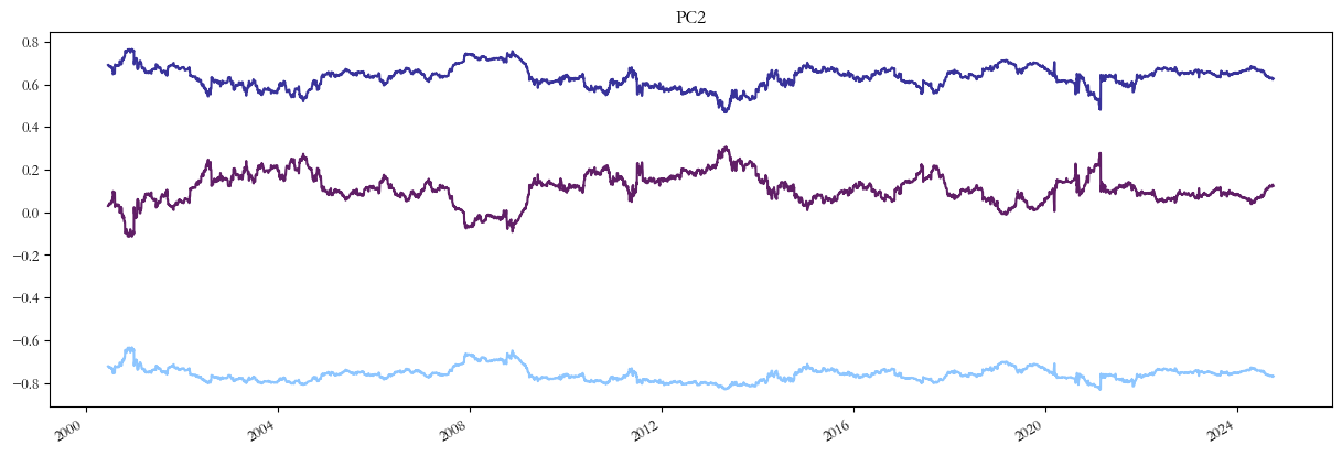
Lastly, the loadings for PC3 correspond to the “curvature” of interest rates. As can be seen below, 2Y and 10Y figures are both positive and tend to interchange for short periods, whereas the belly has a negative sign, resembling butterfly trades.

Trade Implementation

As we are implementing a butterfly trade, we are looking to fully hedge away our exposure against the first two principal components, while maintaining exposure only to the “curvature” one. To do this, we need to use the following matrix inversion formula:

where represents the factor loading associated with the principal component x and the y-years tenor.

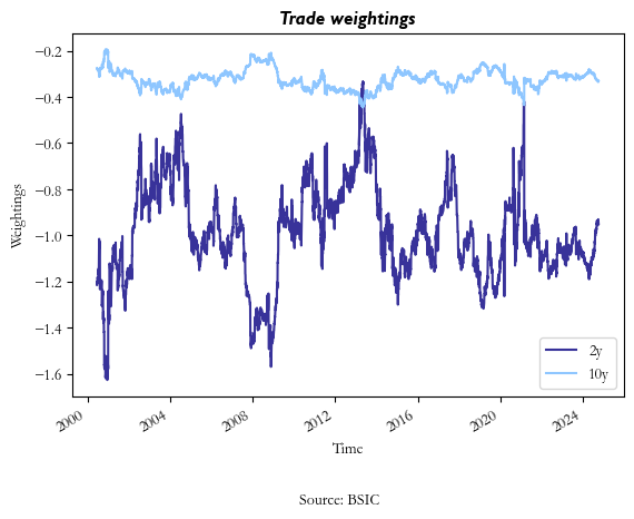
Below it can be visualized how the trade weightings of the 2Y and 10Y legs have adjusted over time considering the changes in factor loadings and DV01. It’s easily noticeable that while the 10Y weighting is mostly contained within a range, the 2Y one is way more volatile, due to a greater adjustment required for its lower duration, but also caused by greater sensitivity changes to the first principal component. It is important to note that the ratios correspond to a 1.0 long position in the 5Y bond.

The evolution of factor loadings presented above was meant to show the relative stability of each tenor’s sensitivity to the three PC, except for when a shift in market dynamics occurs. Consequently, as the market has mostly adjusted to a rates cutting cycle as of now, we will use the most recent loadings to compute the notional values of the trade.

= 0.563, = 0.594, = 0.574, = -0.769, = 0.123 and = 0.626 will results in the two notionals being equal to = -$95.02 million and = -$33.14 million. These amounts are to be shorted in 2Y and 10Y bonds respectively, for every $100 million bought in 5Y bonds.

Conclusion

While we presented two robust statistical approaches for effectively hedging fixed income trades, it is crucial to stress out that the numerical results obtained for the notional values of our trade shouldn’t be taken as granted. First of all, the amounts hedged on each leg should be frequently adjusted, aiming to achieve a good balance between not overpaying transaction costs and being exposed to undesired factors as little as possible. These exposures can stem from changes in betas/factor loadings that are not hedged away in time. Secondly, the statistical properties of the two models presented shouldn’t be the only factor considered when deciding upon a hedging tool. The method adopted should be linked to fundamental factors and the current stage of the monetary cycle. These considerations should be applied to any fixed income trade.

References

1. Tuckman B. & Serrat A., “Fixed Income Securities, Tools for Today’s Markets”
2. Huggins D. & Schaller C., “Fixed Income Relative Value Analysis, A Practitioner’s Guide to the Theory, Tools and Trades”
3. Hirsa A., Klinkert F., Malhotra S. & Holmes R., “Robust Rolling PCA: Managing Time Series and Multiple Dimensions”, March 2023