Introduction
Variance swaps are OTC derivatives that allow investors to get direct exposure to the volatility of an underlying product, such as stock indexes, exchange rates and other asset classes. They initially gained popularity during the early 2000s following the advances in derivatives pricing theory. Their pure exposure to volatility and relative ease of static replication, make them a much more appealing choice for investors and market-makers, as variance swaps do not invoke the additional costs and complexity of delta-hedging or issues with path dependency for the buyers, and hence they have become the preferred instrument used by market practitioners who bet or hedge volatility moves.
In principle, a variance swap is a contract between two parties in which the fixed leg agrees to pay a fixed amount at maturity in exchange for a floating amount based on a realized variance of the underlying. In this article, we aim to explain their pricing method, the main characteristics, and our directional trading strategy.
Pricing
A variance swap is a contract that gives the possibility to speculate on the future (or historical) level of volatility against current implied volatility. You will probably ask why the derivative is based on variance and not volatility. The answer lies in the possibility to easily replicate it, as volatility squared has fundamental theoretical properties, such as additivity.
When a variance swap contract is agreed between two parties, the buyer pays the strike, while the seller pays the realized variance. Thus, the buyer considers that the realized volatility, i. e. the future one, will be higher than the strike, which is fixed at the beginning, such that the net present value of the payoff is zero. The seller, on the other hand, bets that the volatility level for the specific underlying is overpriced.
How to measure realized volatility in a specific period? First, we should mention that volatility is usually calculated on an annual basis, as 252 represents the regular number of trading days in a year, and the logarithmic, rather than arithmetic, returns are considered. Realized volatility can be calculated with the following formula:
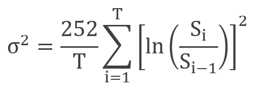
where represents the stock price on a particular day i, and T is the number of days.
The payment amount for a (long) variance swap is given by:
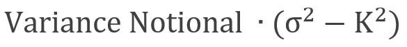
where K is the strike, and variance notional can be written as:
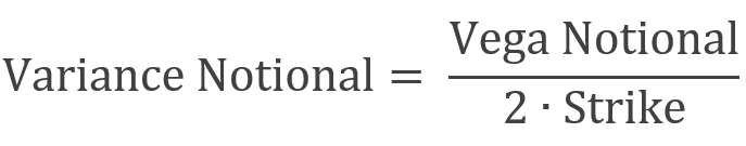
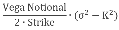
where Vega stands for the notional of a volatility swap. Sometimes we will see the variance swap directly priced with Vega, rather than variance notional, as the former offers a better interpretation of the exposure to the volatility of the party. Thus, the formula of variance swap P&L becomes:
When looking at variance and volatility swaps, you may wonder why their prices differ as they offer similar exposure to volatility. It happens because of the convexity of the variance swaps, which distributes more gains to the buy-side, in the event of an increase in volatility, than losses, given a decrease. Moreover, this phenomenon is highlighted when markets experience increased fluctuations in volatility. Hence, the seller is paid a higher strike. In the case volatility of volatility is close to constant, the variance swap convexity disappears, and its curve tends to become linear. However, the volatility has empirically been non-constant, a pattern that makes variance swap trade above ATM volatility. The price difference is well explained through the presence of skew and skew convexity, which help to achieve implications about the variance swaps pricing.
In fact, if the skew is linear, Demeterfi—Derman—Kamal—Zou obtained a significant relationship between the strike of the variance swap and its skew:
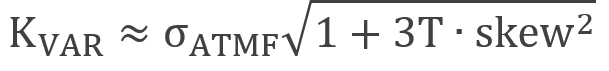
where is the implied volatility of the forward strike, T is the maturity, and skew is the slope of the skew curve. However, this tends to provide better results for short-dated index variance and becomes inaccurate when the skew is steep.
Payoff Convexity
As seen in the previous section, variance swap’s payoff is linear in with variance but convex in volatility. Hence, a long variance swap produces a non-linear profit which is higher than the linear change in volatility and produces a smaller loss for a comparable decrease in volatility. This non-linearity of payoffs is one of the key characteristics of variance swaps.
Similarly to long option positions, the potential loss of a long variance swap is limited, as the maximum loss occurs when the realized volatility is zero, while the inverse is true for short variance swap positions, unless the payout is capped, which we will later come back to. This presence of convexity in the payoff structure is one of the drivers of variance swap levels.
Variance Swap Levels Drivers
In general, the index variance swaps strike levels tend to be above the historic realized volatility, due to their convexity in volatility, which the buyer should pay a fair premium for, and the volatility risk premium, also present in the premia of ATM implied volatilities. However, despite being well correlated, the variance swaps tend to trade even above the ATM volatility levels derived from options, as options volatility represents an estimate around the current price level, while variance swaps give pure exposure to volatility independent of the future market level. In the presence of the skew and skew convexity, deriving a variance strike price from the replicating portfolio of options will usually yield a higher strike level. These effects are more prominent for longer maturity swaps, since for shorter-dated swaps the skew tends to be more linear around the ATM volatility. For shorter-term maturities with relatively linear put skew and flat call skew, we can then use the Derman’s approximation shown in the previous section.
Since the options implied volatility, especially for short-term maturities, is highly correlated to the variance swap levels, we can say that commonly with options volatilities, one of the main drivers for variance swap strikes is historical realized volatility, while the longer dates tend to be more shaped by the macroeconomic outlook and structured product flow. Another important aspect is risk-aversion, as the rising put skews will carry to the swap levels through the channels mentioned above. Finally, volatility tends to be directional and move inversely with the market in the periods of market sell-offs hence driving variance swaps levels inversely to the market levels during market shocks, however, this relationship can change with changing volatility regimes.
Another factor is the volatility risk premium, which describes the phenomenon that on average the variance swaps tend to historically trade above-realized volatilities and due to this bias, the short variance swaps strategies, historically, were on average profitable. This is understandable since the investors are not risk-neutral and agree to pay more for limited downside and a potentially unlimited upside.
Capped vs. uncapped
Coinciding with what we have shown so far, how much more a variance swap is worth due to its payoff convexity depends on how much it is expected to move, thus we can say that the value of the convexity component is based on the expected volatility of volatility, which then, in turn, determines the spread between variance swap and ATM implied volatilities.
These estimates of volatility of volatility aside from being used to price options on variance, also assist in pricing the variance swap caps. Capped variance swap’s payoff can be interpreted as a combination of a long variance swap + writing an OTM variance call. These can be introduced to the trade to limit potential losses for the writer of the variance swap and are usually set at 2.5x strike volatility, thus the value of the cap is relatively small, but the difference in the uncapped and capped strike price should represent the value of the call on variance.
Variance Swap Indices
Variance swaps with different maturities naturally create a term structure, which comparably to the term structures present in e.g. interest rates, can be analyzed by employing similar tools and frameworks used to identify the key factors capturing the variation of the curve.
The volatility indices such as VIX, VXN, VDAX or VSTOXX, are currently calculated using the variance swap pricing methods, producing a theoretical value of a rolling 1-month maturity variance swap based on the prices of traded options, and this change in pricing resulted in the launch of futures on volatility indices in the early 2000s.
In the next section, we will explore a term structure trade idea for the upcoming period.
Trading Idea with Variance Swaps
This year financial markets are experiencing periods of heightened volatility associated to the global Covid-19 pandemic along with other major events such as the upcoming US elections on the 3rd of November and Pelosi’s expected 3 trillion stimulus package. Hence, we believe economic players have been moving to hedge their exposures by buying VIX futures with a particular focus on the short-end. Overtime, this has caused the backwardation of the VIX term structure as you can observe below:
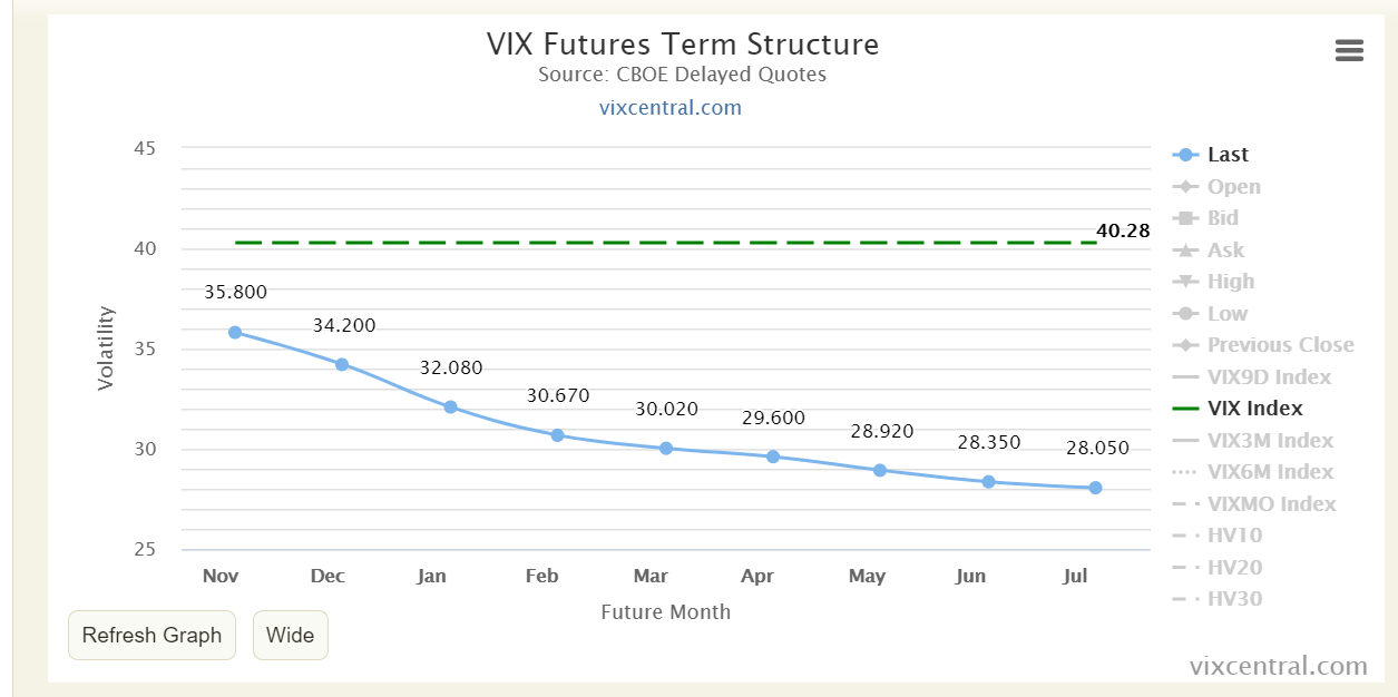
Source: vixcentral
Our view is that the short-end of the VIX curve is too expensive vis-à-vis the long-end, and we expect it to re-adjust as the outcome of US elections becomes clearer for a Democrat win. To take advantage of this opportunity, we could design a strategy using variance swaps and VIX futures as the underlying.
As mentioned extensively above, variance swaps can be useful tools for achieving direct exposure to realised variance without the path-dependency issues associated with delta-hedged options. Therefore, we propose paying 1m/6m VIX variance swap (offering a variance swap on VIX future with a 1-month maturity vs paying a variance swap on VIX future with a 6-month maturity).
Essentially, this means that we expect the realized volatility for the next month ending in December to be lower than the currently priced implied volatility for the same VIX contract. On the other hand, we also expect realized volatility to be higher in the 6 months leg, than the implied volatility for the May contract.
The reasons why we believe the realised volatility in the short-term will be lower than the implied volatility which is at the moment priced in the market is that:
- There was too much protection buying by economic players, making 1-month VIX future too expensive in the curve.
- Risk of a competitive US election is mostly priced in by investors
- 2nd wave of restrictions not as aggressive as previous one at least in the short-term
The reasons why we believe the realised volatility in 6-months’ time will be higher than the implied volatility shown in the market is because:
- The chance that there will be a vaccine in 6-months’ time is quite limited
- Moreover, we believe that the May VIX future looks particularly cheap on its term-structure and hence it is our preferred sector.


0 Comments