The concept of risk parity is not well-known among market participants. However, its resiliency to different market environment makes it a very interesting capital allocation strategy. It was first theorized in the sixties by Ray Dalio – founder of Bridgewater Associates – when he tried to find an answer to the following question: “What kind of investment portfolio would you hold that would perform well across all environments, be it a devaluation or something completely different?” Subsequently, three decades later in 1996, the first fund adopting this particular strategy was introduced. Today “All Weather” Bridgewater’s flagship fund has the stunning amount of $60.7 billion of AuM.
The typical conservative portfolio which is kept by most of retail and also by institutional investors is the 60:40 portfolio: 60% of the capital is invested into bonds and the remaining 40% into stocks. The overall volatility of the portfolio however is mainly related to the equity part as you can see from the following graph. Actual data confirm this: the linear correlation coefficient between SPY and the portfolio is 0.97061577, while between AGG and the portfolio is as low as 0.00981784.
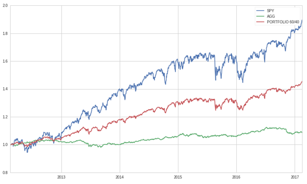
Chart 1: SPY, AGG and Portfolio 60/40 Performance (source of chart data: Bloomberg)
Here we try to explain the underlying concepts of the strategy and we build a risk parity portfolio made of two assets.
We select two assets that are representative of equity and bond market in US. For the equity part we take SPY, which corresponds generally to the price and yield performance of the S&P 500® Index; for the bond part we consider AGG, iShares Core U.S. Aggregate Bond ETF which tracks an index of US investment-grade bonds. Both of them have low expense ratios and are very liquid, thus we can afford to keep them for a long period and we do not have to pay too much in spread cost when we rebalance our position. We plan to rebalance our position once a month so that the weights of the assets reflect new measures of volatility.
The basic idea behind a risk parity portfolio is that each asset contributes in the same way to the portfolio’s overall volatility. In this case, given that we have only two asset, 50% of the portfolio risk comes from equity, the remaining 50% from bonds. We base our model on the mathematical solution provided by Maillard and Roncalli, who find the optimal weight distribution as the solution of a minimization problem. Here we extract only the relevant part, not all passages are stated. For a more analytical approach check their paper “On the properties of equally-weighted risk contributions portfolios” (Maillard, Roncalli 2009).
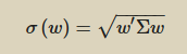
The volatility of the portfolio is defined as:
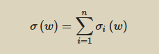
The risk contribution of asset i is computed as follows:
![]()
You can then show that:
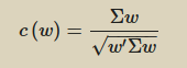
The vector of the marginal contributions is computed as follows:
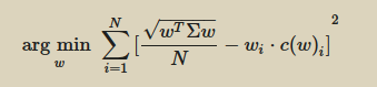
And finally we can find the weight to assign to each asset by minimizing the following function:
We run our algorithm every 6 months to find the updated weights. For our calculations and for the sake of simplicity we do not use rolling variables such as rolling correlation or rolling variance. Instead we take a 5 year window, we split it into 10 parts and consider them individually. Weights obtained in this way are shown in the table hereunder. You can see that when bond volatility goes up, we allocate more capital to equity and vice versa.
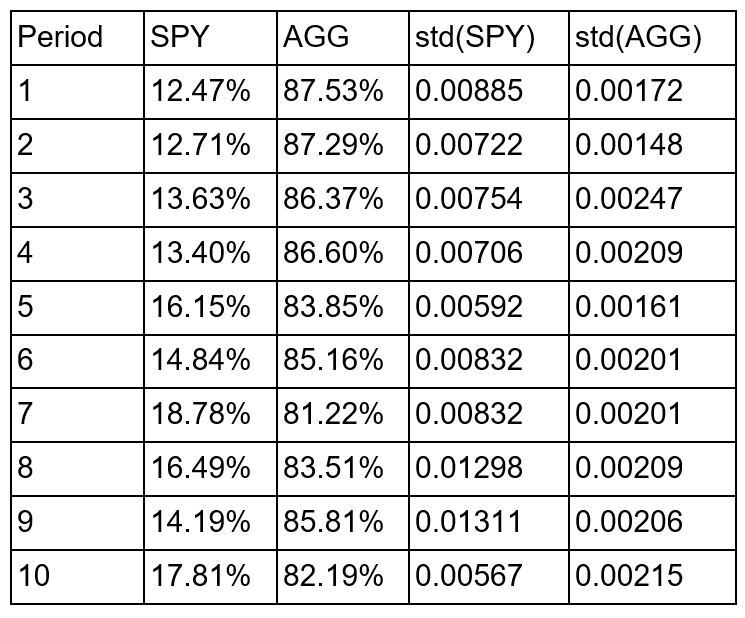
Table 1: SPY-AGG allocation vs volatilities (source of chart data: Bloomberg)
Now that we know the weights, we can see how our risk-parity portfolio performs over the same period. Given that we are in a portfolio theory environment we assume that there are no transaction costs and that the bid-ask spread is zero. Differently, we consider the expense ratio for both the ETFs, which is 0.10% yearly for SPY and 0.06% yearly for AGG. In the next graph we can see a comparison between the portfolio made of 60:40 bond-equity and our risk parity portfolio, which allocates the risk 50:50 to bond and equity, resulting in a 85:15 average allocation.
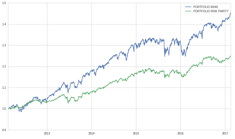
Chart 2: Portfolio 60/40 vs Portfolio Risk-Parity Performance (source of chart data: Bloomberg)
As we could expect, the risk parity portfolio has lower return than its counterpart, since the former is composed mainly by bonds, so how come that so much money is deployed through this strategy? How can we make this strategy more profitable? Well, we can leverage our risk parity portfolio, and that’s exactly what the majority of other market players adopting this strategy does, Bridgewater Associates included.
This infographic comes from a research from PanAgora Asset Management and plots the suggested relationship between leverage ratio (y-axis), linear correlation coefficient and diversification return (x-axis).
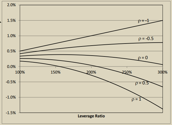
Chart 3: Leverage ratio vs correlation coefficient vs diversification return (source : PanAgora Asset Management)
According to these data, the recommended level of leverage for this particular strategy in order to maximize expected return of the portfolio made of these two ETFs will be between 200-220%, which is very high, but not uncommon for these kind of portfolios. As always, proceed with due diligence before engaging in risky investments with high leverage.


0 Comments