If volatility be rough with you, be rough with volatility

Download as PDF

The purpose of this special report is to introduce the emerging class of rough volatility models. Rough volatility is a relatively new concept originating from the empirical observation that log-volatility essentially behaves as a fractional Brownian motion at any reasonable timescale. While rough volatility is found to have increased accuracy and predictive power with respect to existing models, its modelling peculiarities make numerical implementations more computationally expensive, limiting its practicality. Recent developments, notably the work of Horvath, Mugurunza and Tomas [1] have greatly advanced numerical implementations, thus heralding a possible adoption in the industry.

First a brief introduction of traditional stochastic volatility models is presented, then rough volatility is introduced together with fractional Brownian Motions, finally the numerical implementation based on neural networks of Horvath et al. is presented and replicated.

Introduction

Despite its popularity, the Black-Scholes model has well-known shortcomings, not least with respect to volatility, which is assumed to be either constant or a deterministic function of time. After the appearance of the volatility smile, a number of models were developed to account for the new dynamics of the market and allow for consistent pricing of derivatives.

A popular approach is to model volatility as a stochastic process, where the choice of the specific dynamics define the model. Since their introduction, stochastic volatility (SV) models have grown both in popularity and complexity. Notable examples are the Heston model, SABR, Hull and White, and Bergomi model. Each model has its own peculiarities and depending on the pricing needs one might be preferred over the others. As an example, the Heston model has the following dynamics:

(underlying)

(volatility)

Where the required correlation between underlying and volatility is achieved by correlating the two Brownian motions, .

Fractional Brownian motions and Rough Volatility

First of all, a technical note. Rough volatility models employ a more general concept of the usual Brownian motion, called fractional Brownian motion (fBm). The key difference is that the increments of a fBm need not be independent and in particular the covariance is

where the parameter H is called Hurst parameter and drives the raggedness of the process:

1. If , the increments are negatively correlated
2. If , the increments are positively correlated
3. If , the increments are independent and we retrieve the classical Brownian motion

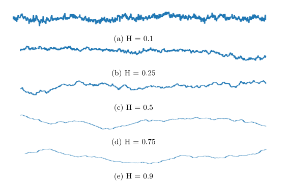
Figure 1: Sample paths of fBm for different values of the Hurst parameter

Fractional Brownian motions were first employed in volatility modelling by Comte and Renault [2]. Their model used a fBM with H>1/2 (positively correlated increments) to model volatility as a long-memory process i.e. one where autocorrelation decays slowly – a widely accepted stylized fact. They thus introduced the class of Fractional Stochastic volatility models.

However, their model however generates data which is inconsistent to what is observed in the market, in particular with respect to the ATM skew:

where and .  Indeed, the model of [2] generates a term structure of the ATM skew which is increasing in time, while empirically we observe an “explosion” for short maturities and then a decay, well approximated by a power law.

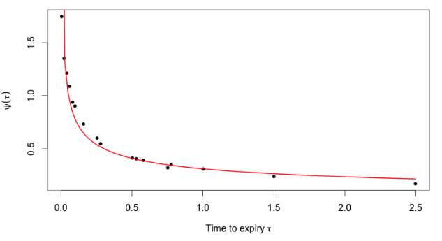
Figure 2: From [3]. The black dots are non-parametric estimates of the S&P ATM volatility skews as of June 20, 2013; the red curve is the power-law fit

Moreover, the overall shape of the volatility surface in equity markets does not change over time, at least to a first approximation. This makes it desirable to have time-independent parameters for the volatility process. However, existing time-independent stochastic volatility models also fail to properly fit they skew. Indeed, they generate a constant ATM skew for short maturities, again inconsistent with what is observed in the market.

It was common belief that to replicate such “explosive” features it was necessary to introduce jumps. However, Fukasawa [3] showed a fBm with Hurst parameter H would imply an ATM skew in the form of . But then to replicate what is observed in the market it was necessary to have H<1/2, apparently losing the long-memory features that first prompted Comte and Renault to use the fBm.

Following these observations, Gatheral et al. [4] define volatility as “rough” i.e. as driven by a fBm with H < 1/2, thus introducing the class of Rough Fractional Stochastic Volatility (RFSV) models. In particular, they first employ an empirical estimation to assess the smoothness of the volatility process, using realized variances estimates across the main stock indices. They find two main regularities. First, a consistent mono-fractal scaling relationship for log-volatility, with smoothness factor H in the order of 0.15. Second, an approximately Gaussian distribution of increments of log-volatility, consistent with previous studies. Overall, this suggests the modelling of log-volatility with a fBm, similar to the one used in Comte and Renault but with H < 1/2.

A couple of remarkable features of this model are worth mentioning. First, RFSV forecasting is found to be as good as other established volatility forecasting techniques (e.g. HAR) but with fewer parameters. Second, despite the negative correlation of increments (H < 1/2), RSFV-generated volatility “fools” standard techniques in financial econometrics, which tend to find in it spurious evidence of long-memory.

Overall, there seems to be a consensus that rough volatility is the way forward for volatility research. The seminal paper by Gatheral et al. spurred intense research in the field, roughly divided in two main areas. The first area is theoretical, “roughening” existing stochastic volatility models with the new machinery of rough volatility (e.g. rough Heston). The other area is empirical and will be further explored in the next section.

Simulating rough volatility

Despite their increasing popularity since they were first introduced in 2014, rough volatility models have so far found little adoption in the industry. The main reason lies in their numerical (in)tractability. Indeed, the enhanced features allowed by the fBm come at a cost, namely Markovianity, which is lost together with easily derivable closed-form solutions. This in turn implies that calibrations need to rely on expensive Monte Carlo simulations, making practical usability almost null.

To make the point clearer, think about how calibration usually works. Imagine that you have a model with parameter space and a set of market data relevant for calibration. The model is effectively a pricing map, taking as input a parameter combination and the specific details of the derivative to be priced (strike, maturity etc.) and giving as output its fair price. In its crudest form calibration essentially boils down to a repeated evaluation of the pricing map for different combinations of parameters, until a sufficient precision is achieved. To sum up the procedure:

1. Select a specific parameter combination
2. Evaluate the prices using the parameter combination of step1
3. Compare the output of step2 with the actual market data. If a sufficient precision is achieved, stop. If not, restart from step1 with a different parameter combination.

Now, call N the total number of evaluations needed to achieve a decent precision. If the pricing map is available in closed form, then step2 is very fast and calibration can be done in reasonable time frames even for a large N. If a closed form is not available, as tends to be the case for rough volatility models, step2 itself becomes a numerical process, where to evaluate the prices we need to use a numerical simulation. This is where the non-Markovianity of rough volatility kicks in, since it makes the numerical evaluations of step2 very slow and effectively prevents industry adoption.

Addressing this issue, researchers have put forward methods to speed the simulation. Some examples are: Cholesky decomposition methods, variance reduction techniques such as antithetic sampling and control variates, and neural networks. It is this latter approach, due the joint work of Horvath, Muguruza and Tomas [1] (recipients of the Risk Magazine 2020 award “Rising star in quant finance”) that is briefly summarized here.

This approach solves the bottleneck by splitting calibration in two parts. The first part is an offline procedure to learn the pricing map using a neural network. That is, mapping model parameters to pricing functions (implied volatilities). Once the NN is trained, the second part consists in using the (now deterministic) pricing map to compute the actual calibration, which is completed in a matter of seconds. In other words: the NN first learns how different model parameters would translate to prices. This is procedure is lengthy, computationally expensive and is done offline. Once the model is trained, the pricing map becomes effectively a deterministic map so the actual online calibration can be done in a matter of seconds – following step 1,2,3 above.

The authors carry out a thorough review of network architectures and objective functions, finally setting on an image-based implicit learning. It borrows from established image recognition techniques and essentially amounts to designing the pricing map to store the implied volatility surface as an image with a grid of “pixels” (read: combination of strikes and maturities) which can be made arbitrarily fine.

Figure 3: Surface to 2d grid

Implementation and results

Following the work in [1], we report here a numerical implementation. The specific model chosen is the rough Bergomi model with flat forward variance, for a thorough review of the model see [5].

The model has four parameters including the initial forward variance, the Hurst parameter, and the correlation between the underlying and volatility processes. The volatility surface is converted in a matrix of 8 maturities and 11 strikes. The NN has three hidden layers with 30 nodes each and is trained on 40.000 parameters combination.

The training takes up the most part, around 5 minutes on a standard laptop in this simple setting – in practice this will be relegated to an offline procedure. The actual online calibration is very fast, in the order of milliseconds, and relatively accurate.

Note: Code was implemented with Python using Keras for the NN and Scipy for the calibration, based on the original code provided by the authors and freely available on Github. Calibration is done to an arbitrarily chosen market state.

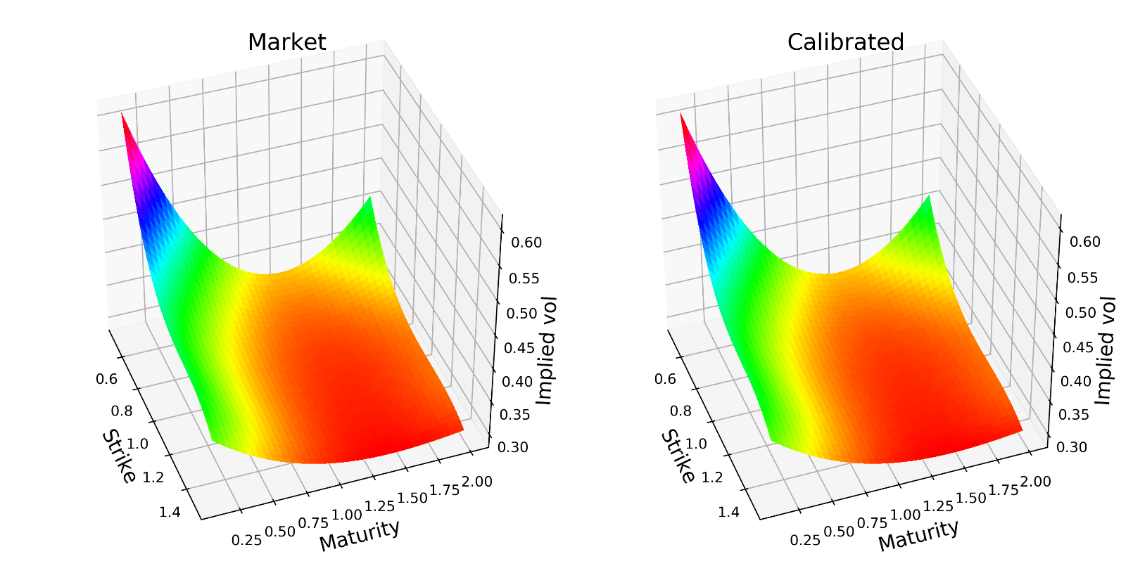
Figure 4: Market vs. calibrated volatility surfaces

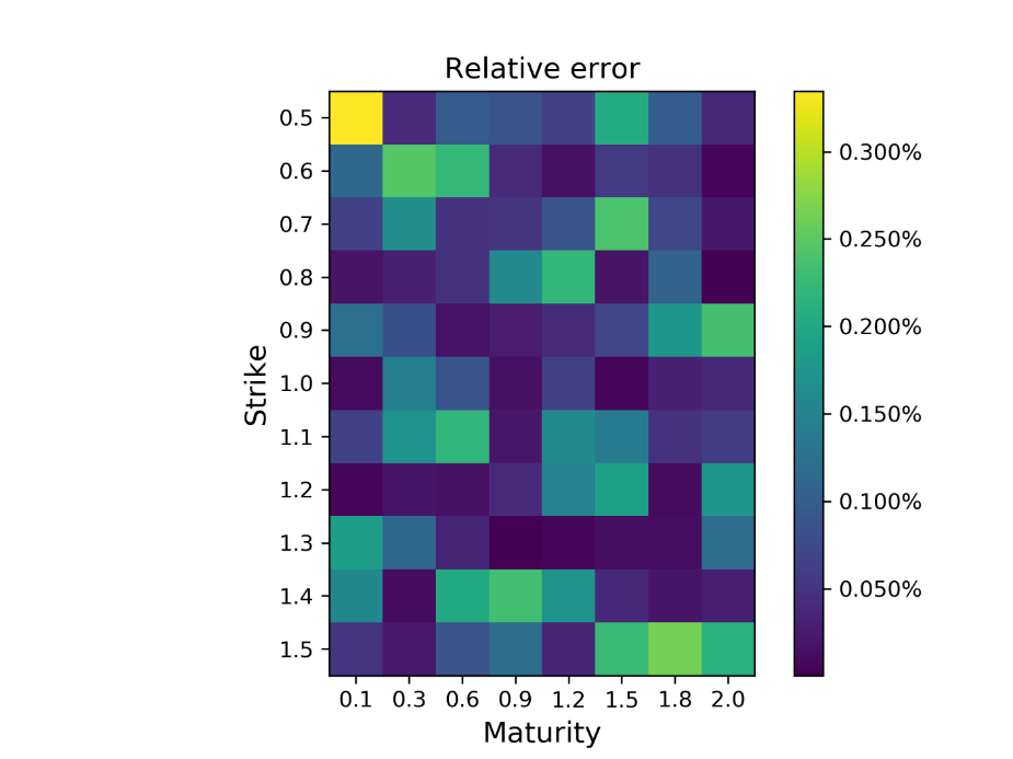
Figure 5: Relative errors on the 11×8 grid

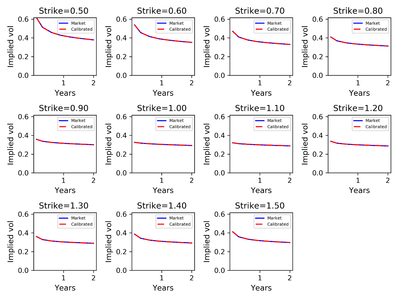
Figure 6:  Term structure for each strike

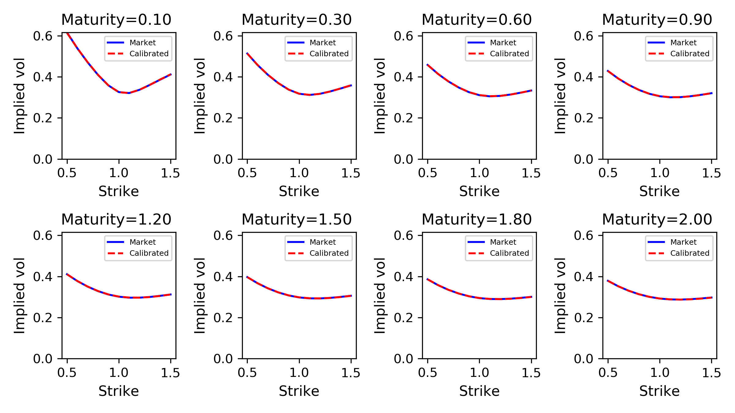
Figure 7: Smiles for each maturity

Sources

[1] “Deep learning volatility”, Horvath, Muguruza, and Tomas

[2] “Long memory in continuous-time stochastic volatility models”, Comte and Renault

[3] “Asymptotic analysis for stochastic volatility: martingale expansion”, Fukasawa

[4] “Volatility is rough”, Gatheral

[5] “Pricing under rough volatility”, Bayer, Fritz, and Gatheral