Introduction
In this article, we discuss an equity Pairs Trading strategy using the S&P 500 index components. Pairs Trading is a statistical arbitrage strategy that involves simultaneously taking long and short positions in two financial assets, expecting their spread to converge to the mean. However, the process of identifying the most profitable pairs of securities in a high-dimensional context can be a complex task, both from a statistical and a computational point of view. For this reason, we adopt the sparse Gaussian model known as Graphical LASSO (GLASSO), which computes the precision matrix of the stock returns and acts as a filter in the pairs identification phase, thus accelerating the process. Finally, we backtest the strategy, analyze its excess returns and its risk factors exposures.
Pairs Trading
Pairs Trading is a statistical arbitrage strategy that aims to achieve excess returns by exploiting mean-reverting statistical relations between pairs of securities. For an introduction to this strategy, see here and here. In short, two stocks  and
and  should be traded when cointegrated, that is when there exists a spread
  which is stationary over time, hence mean-reverting. There are different ways to obtain such
  , which include – but are not limited to – Ordinary Least Squares (OLS) regression of on , rolling OLS regressions, and the so-called Kalman Filter. An important feature of is to be a time-varying estimate, so the former regression method is usually discarded. To test for cointegration, we perform the augmented Engle-Granger two-step cointegration test, where the null hypothesis is the absence of cointegration.
Once a pair of cointegrated stocks is identified, the strategy can thus be executed. First, the spread is standardized, and a certain threshold of the standardized spread is identified as the entry point of the trade. The trade is constituted by a long and a short leg, and to achieve market neutrality the quantity bought of stock  is always
  times the one of
  . Then, the spread is expected to converge to the mean and, when it does so, the trade is closed with a profit.
Example (with an entry point at 2 standard deviations from the mean):
 : SHORT Y, LONG X, spread is expected to decrease;
 : LONG Y, SHORT X, spread is expected to increase.
Nevertheless, the spread might diverge from its mean due to a regime shift in the cointegration between the stocks, in which case the trade should be closed immediately, even without a profit. To account for this, another level of the standardized spread is identified as a stop loss. A possible modification to this trading system is to adjust the size of the position on the pair depending on the spread itself – increasing while farther out from the mean and vice versa – without the need to identify an arbitrary entry point threshold. However, this new mechanism might be difficult to implement as overtrading and dynamic risk exposures might increase dramatically transaction costs.
The calculation of returns of a cash-neutral strategy such as Pairs Trading is a complex task which does not come in a standardized form. We adopt two different methods, that is to divide the long-short profits by the long leg plus the additional margin requirement of the short leg, or just by the additional margin requirement. We denote the first method by “Both Legs” (B.L.), and the second by “Margin Only” (M.O.). In the former case, we are assuming that the investor must leave the short sell proceeds in a broker’s account, while in the latter the investor can use the short sell proceeds to fund the long position. Clearly, returns calculated with the second method will be higher. Without loss of generality, assume that we are going long on and short on as stated above, daily returns are calculated according to the following formulas:


here  is the initial margin required for the short position once the stock is sold short on the market. It is important to note that the formula is simplified and cannot be replicated in a live trading environment without considering factors such as variation margin (variable to each exchange’s policy), negative carry from financing costs and dividend payments during the trade. In our analysis, we will also use past data of bid-ask prices for each stock to account for transaction costs, considering bid-ask spread skewness.
The Case for GLASSO
In many financial problems it is crucial to understand the relations between different assets, which are usually measured with correlation. Nevertheless, if two assets belong to the same index (as in our case, for two stocks of the S&P 500), they might possess a strong spurious correlation which is not explained by any economic rationale. This is due to their common correlation with the index they belong to: the so-called market beta, that acts as a confounding variable. Partial correlation instead determines the association between two time series after removing a set of confounding variables, which in this case are all the other securities in the index, thus obtaining an estimate which exploits the idiosyncratic relationship between two stocks. Partial correlations are derived from the precision matrix  of the observations i.e., the inverse of the covariance matrix
  , through the following formula:

where  is the partial correlations matrix.
GLASSO is a statistical method used for estimating sparse precision matrices of normally distributed random variables in high-dimensional settings. In its approach, we combine two important concepts: the graphical modelling of conditional dependencies between variables and the L1 penalization of the Maximum Likelihood Estimator (MLE). The method solves a convex optimization problem with a penalty term  that encourages sparsity in the matrix. This sparsity assumption enables the identification of important relationships between variables while ignoring irrelevant connections. The resulting estimate is represented as a graph, where nodes correspond to variables, and edges represent conditional dependence relationships, that is non-zero partial correlations. The GLASSO method is commonly used in applications such as gene expression analysis, brain imaging, and financial portfolio optimization, where the number of variables is large, and the underlying network structure is unknown.
In mathematical terms, GLASSO aims at solving the penalized Maximum Likelihood Estimation problem:

where  means that we optimize over positive semi-definite matrices,
  is the determinant operator,
  is
is  , and the last term is the penalization, obtained by multiplying the penalization parameter , which controls for the sparsity level of the precision matrix, by the L1 norm of the off-diagonal entries, that is
  . The problem is endowed with some theoretical guarantees such as convexity, the existence of a global minimum, and the symmetry of
  . Cross-validation and eBIC are two popular techniques to fine-tune the parameter .
One of the main issues of the Pairs Trading strategies arises during the pairs identification phase, when possibly each pair of stocks should be checked for cointegration. As the number of pairs to test scales quadratically with the number of index components, for indexes with thousands of components it might be infeasible to perform millions of hypothesis tests and regressions. Another problem is that, when dealing with high-dimensional data, it is common to encounter pairs that have a statistically significant relationship not explained by any economic rationale, that for instance might be presence due to the multiple testing bias. The contribution of GLASSO is twofold: it provides a way to test only a subset of pairs, that is the ones connected in the graph, and it usually does so by identifying clusters of stocks grouped by sectors, partially explaining the economic rationale.
Our GLASSO-based Pairs Trading Strategy
For our purpose at hand, we use the S&P 500 index with the daily Bid and Ask of each component, ranging from 2018 to 2022. Moreover, we also need the sectors of each stock to check whether GLASSO groups stocks in different sectors clusters. Since the main assumption of GLASSO is that the input data follows a multivariate normal distribution, we proceed to perform the Shapiro-Wilk normality test with significance level of 0.01 on the weekly log-returns, as proposed by Mota (2012).
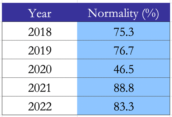
Figure 1. Percentage of weekly log-returns that do not reject the normality hypothesis each year.
Source: Bocconi Students Investment Club
On average, the vast majority of stocks do not reject the normality hypothesis. In 2020, due to high market volatility and frequent tail events, the normal distribution did not manage to fit most of the stock returns. To feed the data into GLASSO we standardize weekly log returns before calculating their covariance matrix over the period 2018-2020, as proposed by Robot Wealth (2020). Next, we run GLASSO on the covariance matrix with the penalization parameter  , since we find this value of the parameter to yield a feasible number of pairs and to divide stocks into sectors group.
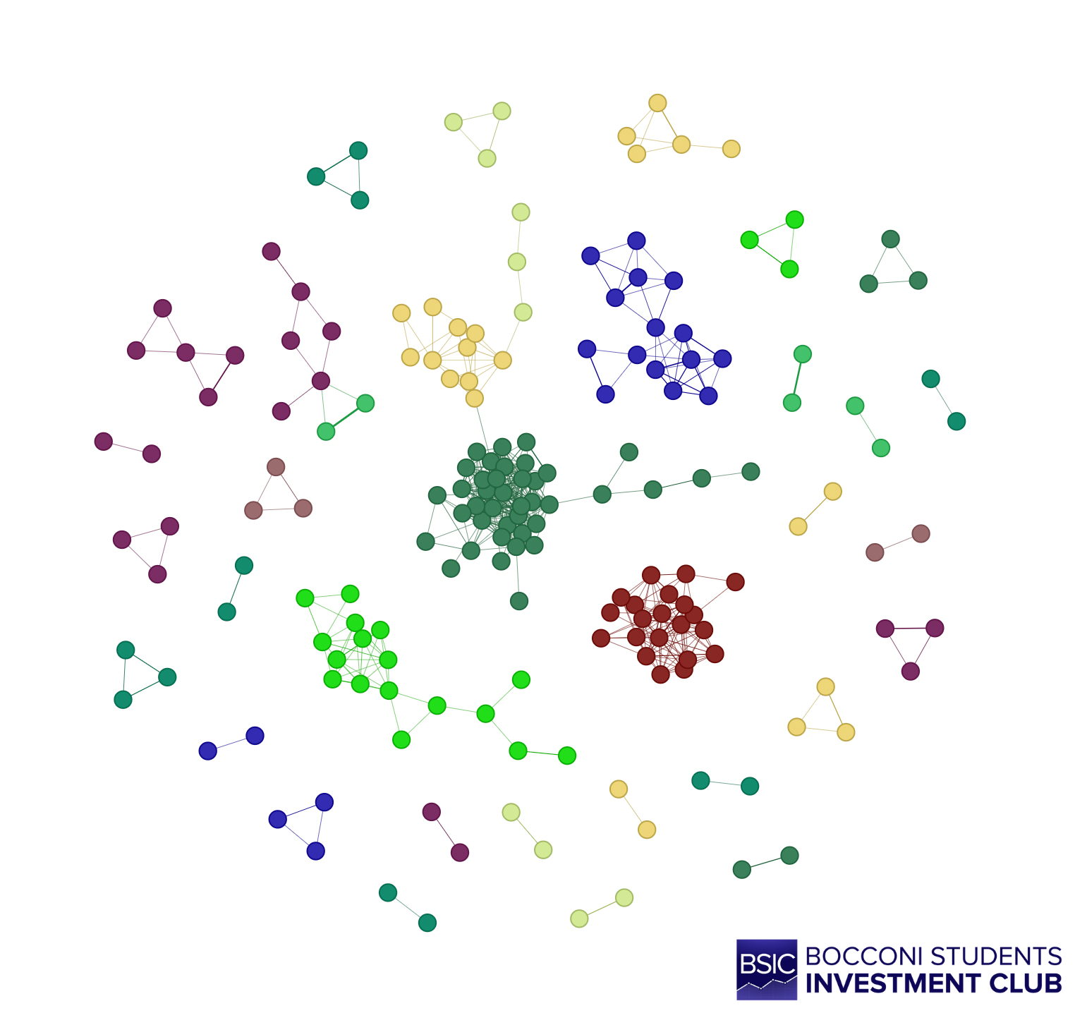
Figure 2. Graph of partial correlations, stocks are colored according to their sector.
Source: Bocconi Students Investment Club
As you can see from the graph above, sector clusters are formed within stocks, the most evident ones being Financials (dark green), Energy (lime), Utilities (dark red), and Real Estate (dark blue). For each pair identified by the GLASSO, we run an Engle-Granger cointegration test with a significance level of 0.05 over the same period. This step acts as an additional filter, reducing the number of pairs from 512 to 38.
After having identified all the pairs, we run the trading strategy from 2021 to 2022, so that the trading period does not overlap with the GLASSO period. The spread  between two cointegrated stocks is built with the of a rolling OLS regression of on with a rolling window of 30 days, and it is then standardized on a rolling standardization window of 60 days. The entry point of the trade is set at 2 standard deviations. As for the returns calculation, we employ the two aforementioned methods, with an initial margin requirement set at 150%, i.e. the full short sell proceeds plus an additional margin of 50% of the value of the short position.
The cumulative returns over the trading period are respectively 17,2% for the M.O. strategy and 5,5% for B.L. Statistical Arbitrage strategies usually have a higher Sharpe Ratio compared to the market, due to their low volatility. According to Gatev (2006), the Sharpe Ratio can be from 4 to 6 times the one of the S&P 500. In our case the M.O. strategy achieves a Sharpe ratio of 1.91, while B.L. 1.46.
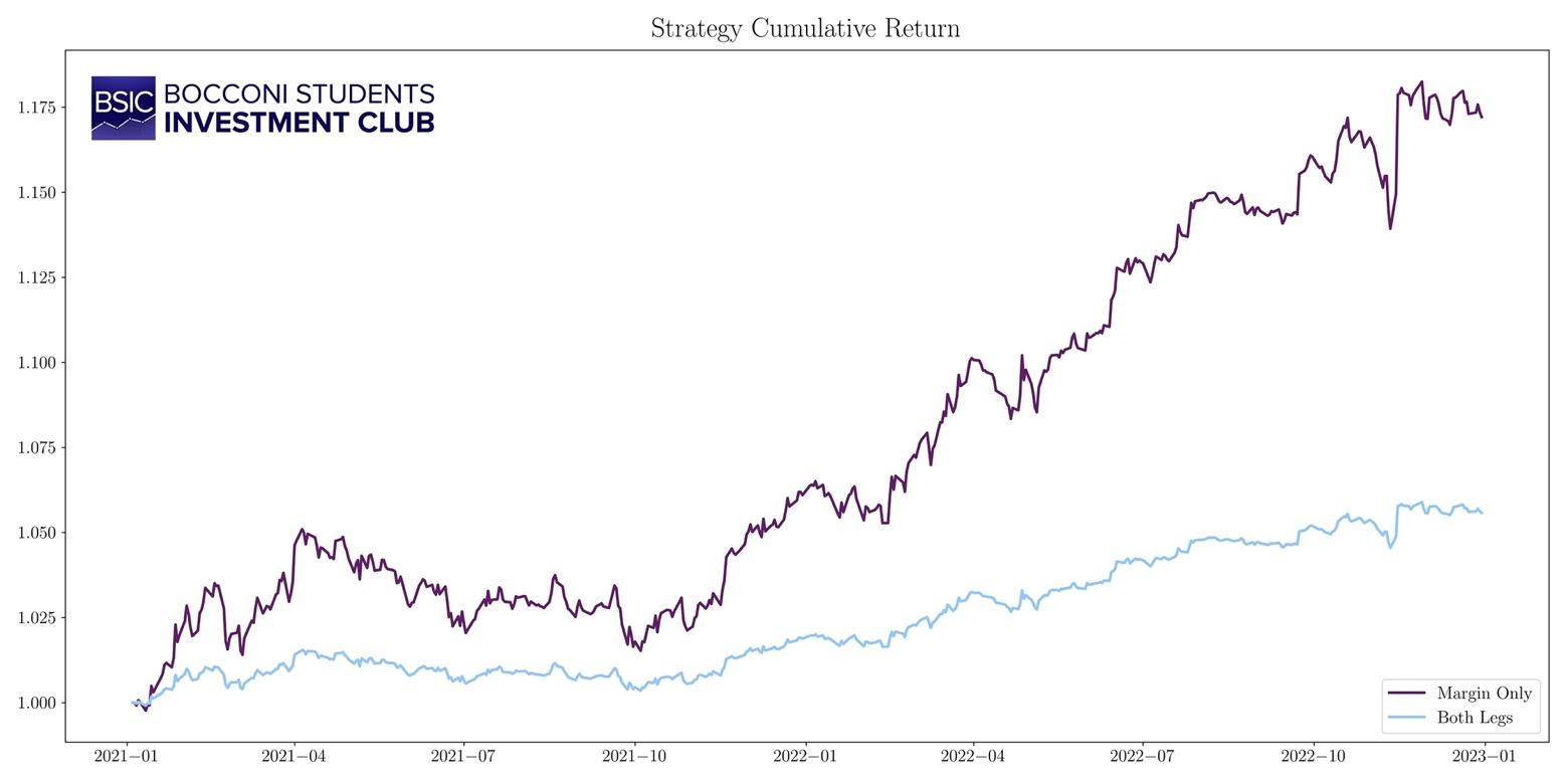
Figure 3. Cumulative returns.
Source: Bocconi Students Investment Club
By analyzing the return distribution, we observe two common characteristics of mean-reversion strategies (see Gatev, 2006), that is positive skewness and excess kurtosis, which are respectively 1.3 and 7.0. This means that frequent small losses and few large gains tend to occur.
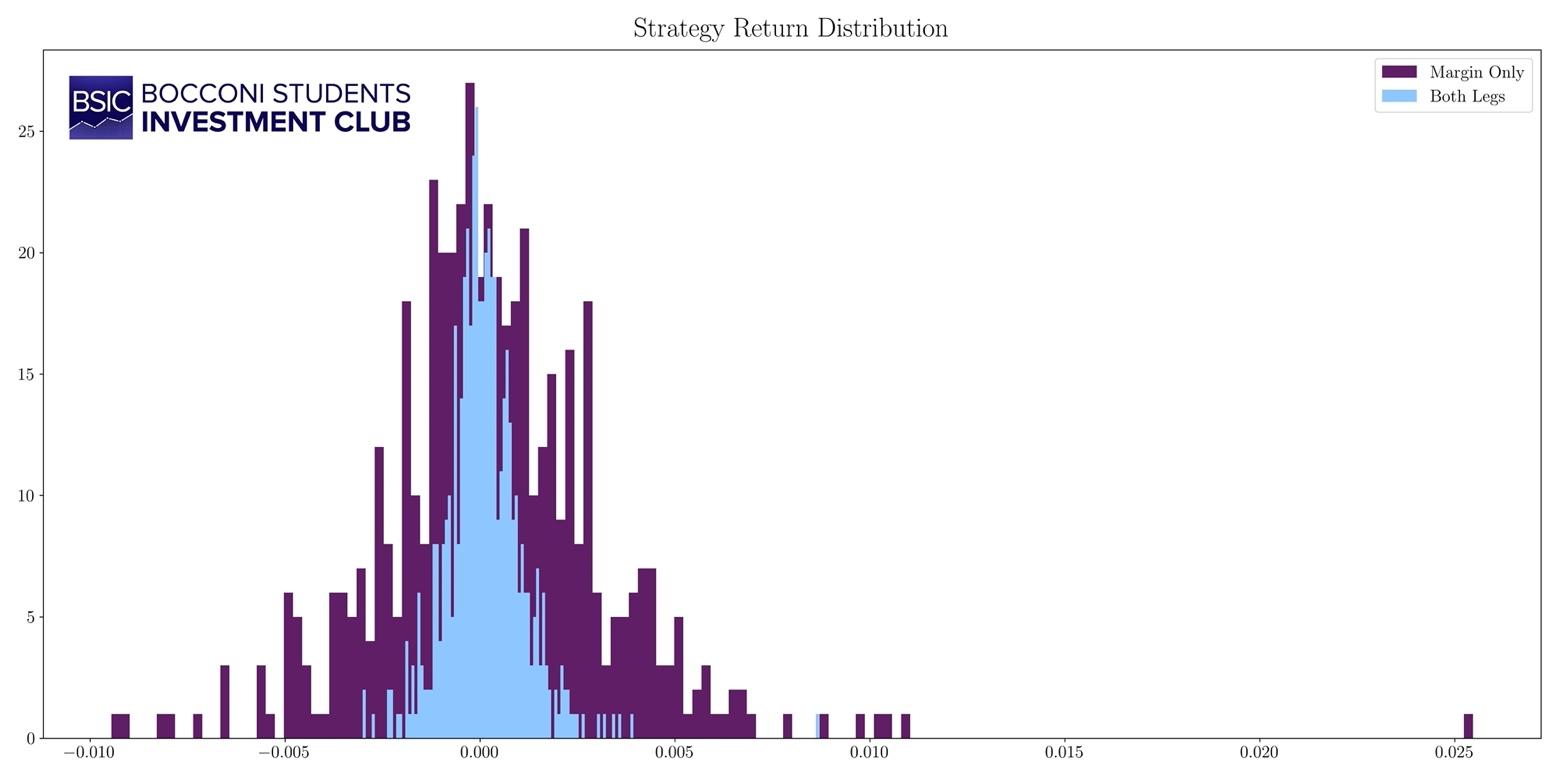 Figure 4. Probability distribution of returns.
Source: Bocconi Students Investment Club
Since our Pairs Trading strategy must be market-neutral, we test for market-neutrality by regressing the strategy returns on the market returns, finding that the market beta is statistically insignificant.
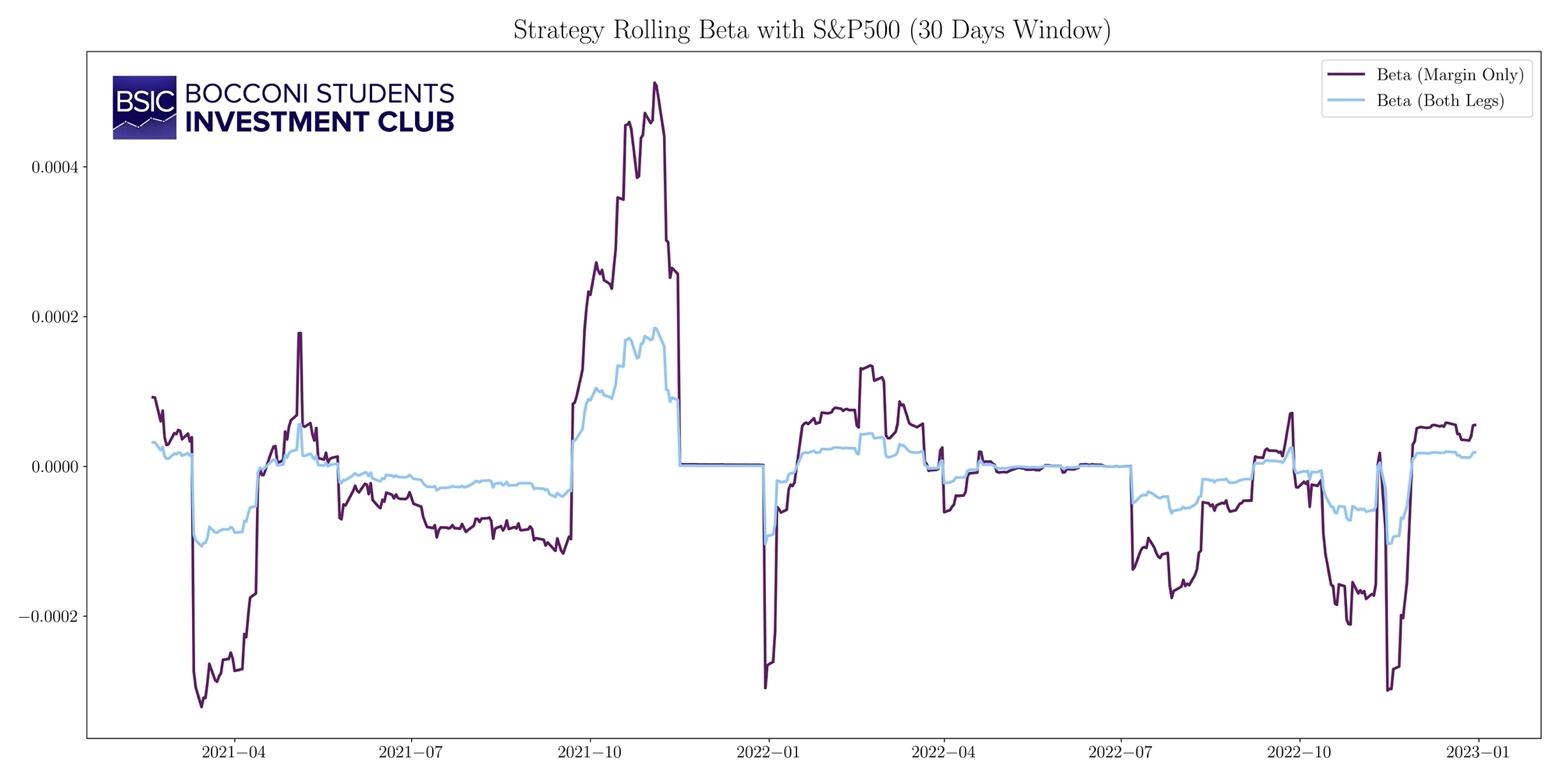
Figure 5. Rolling market beta (30 days window).
Source: Bocconi Students Investment Club
Crucially, we proceed with a factor analysis of our systematic strategy. The importance of this analysis is encapsulated by the need to understand whether the strategy generates abnormal returns or simply harvests risk premia. We can observe that, testing our strategy’s monthly excess returns against the 3 Fama-French factors – Mkt-RF as market excess return, SMB as Small-Minus-Big, HML as High-Minus-Low – as well as the Momentum factor, the regressions yield similar results with the two return calculation methods. Indeed, it is evident that any factor exposure is statistically insignificant, arguing in favor of our factor-neutral portfolio argument. The intercept of the regression, i.e. the alpha of the strategy, is significant and has a value of 0.8% for the M.O. method and 0.2% for the B.L. method. We note that the Momentum factor rightfully shows a negative coefficient, as Pairs Trading falls under the umbrella of mean reversion strategies. Finally, a low  of 0.12 (M.O.) and 0.11 (B.L) argues again in favour of our thesis.
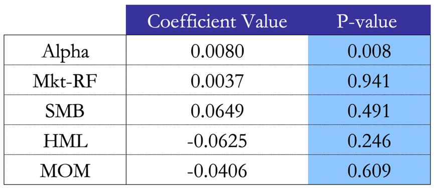
Figure 6. Factor regression results with the M.O. method.
Source: Bocconi Students Investment Club
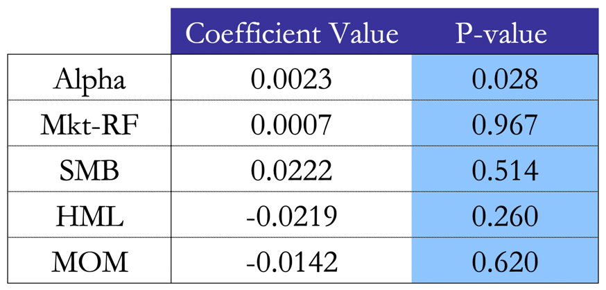
Figure 7. Factor regression results with the B.L. method.
Source: Bocconi Students Investment Club
Limitations of the Study and Possible Improvements
To conclude, Pairs Trading is a statistically robust strategy that yields excess returns when tested against the well-known Fama-French factors. On one hand, GLASSO helps us to identify the suitable pairs by estimating sparse precision matrices of normally distributed random variables in high-dimensional settings. On the other, our modelling of the transaction costs gives a reasonable estimate on the sustainability of a strategy with a margin cost, a potentially high turnover and a systematic, yet tailored way to seek entrance/exit trading thresholds.
However, as a further potential improvement, we note that we have assessed the optimal for the GLASSO for the period 2018-2020 and we used that value and pairs for the trading period 2021-2022. It goes without saying that a live trading strategy should rely on a backtesting infrastructure which supports a rolling GLASSO technique, whereby pairs are promptly tested against a potentially changing market regime as new market data comes in. Among other things, live trading and backtesting this strategy outside of our simulated environment should require strengthened methods checking for the cost of borrowing money, the negative carry, the arising possibility of margin calls as well as the dividends due from the shorted leg of the portfolio.
Ultimately, as per Gatev (2006), there are some limitations in this study which are worth a mention. Firstly, the paper argues that a latent factor is behind the Pairs Trading phenomenon. Namely, such latent risk factor could have a strong theoretical link with the Law of One Price (LOP): Ingersoll (1987) defines the LOP as the “proposition … that two investments with the same payoff in every state of nature must have the same current value”. Chen and Knez (1995) extend this to argue that “closely integrated markets should assign to similar payoffs prices that are close”. Secondly, sensitivity of the Pairs Trading to the default premium suggests that the strategy may work because we are pairing two firms, the first of which may have a constant or decreasing probability of bankruptcy (short end), while the second may have a temporarily increasing probability of bankruptcy (long end).
Yet most importantly, as Jegadeesh (1990) and Lehmann (1990) argue, it is left to show that Pairs Trading is simply not a negative autocorrelation strategy. Indeed, while it is correct that our strategy is negatively correlated with momentum, it is left to show that our returns are positively correlated with – but not explained by – the short-term reversals factor. Furthermore, the nature of our excess returns is aligned with the academic and practical research analyses: generally skewed right and with positive excess kurtosis relative to a normal distribution. The conclusion is that Pairs Trading is profitable in every broad sector category, and not limited to a particular sector.
Sources
- Schmidt-Hieber. “Lecture Notes”.
- Robot Wealth, 2020. “The Graphical Lasso and its Financial Applications”.
- Pei, 2017. “An Elementary Introduction to Kalman Filtering”.
- J. P. Broussard, M. Vaihekoski, 2012. “Profitability of Pairs Trading in an Illiquid Market with Multiple Share Classes”.
- Mota, 2012. “The Shapiro-Wilk and related tests for normality”.
- Mazumder, Hastie, 2011. “The Graphical Lasso: New Insights and Alternatives”.
- Gatev E., Goetzmann W., Rouwenhorst K., 2006. “Pairs Trading: Performance of a Relative Value Arbitrage Rule”.
- Chen and Knez, 1995. “Measurement of Market Integration and Arbitrage”.
- Jegadeesh, 1990. “Evidence of Predictable Behavior of Security Returns”.
- Ingersoll, 1987. “Theory of financial decision making”.


0 Comments