The Death of FX Volatility, What’s Next?

Download as PDF

Introduction

Over the past few years, volatility in the foreign exchange markets has entered a marked downward trend, which ultimately culminated with the signing of the US-China Phase One trade deal in January 2020. This descending movement has characterised both Developed and Emerging Markets currency pairs and was largely driven by a macroeconomic environment in which central banks’ easier monetary policies play the lion’s role. Indeed, as a result of the excess liquidity in the markets, not only we observe an unprecedented low FX volatility but also price swings across all major asset classes have been suppressed.

In this article, after having provided an overview of the recent behaviours of realised and implied volatility in the foreign exchange markets, we discuss some of the possible economic explanations for such trends, trying to assess whether the low FX volatility phenomenon is likely to persist in the short/medium term. Then, aiming attention at the EUR/USD exchange ratio, we investigate the effects of some macroeconomic factors on its volatility through a simple GARCH model.

The Low Volatility Environment in Foreign Exchange Markets

As an introduction to the volatility environment of FX markets, we would like to explain what we refer to when we talk about volatility. As in all financial assets, there are two types of volatility that can be observed in Foreign Exchange markets: historical (realised) and implied volatility. Realised volatility is always calculated for a certain time periods (i.e. 3 month realised volatility, 9 month realised volatility) and refers to the standard deviation of returns of a financial security within that time period. While realised volatility can be calculated using historical returns, implied volatility must be extracted from option prices. Implied volatility is particularly useful as it is a factor which can show the sentiment of option market participants towards the given security’s future volatility. It is also important to note that moneyness and option type affect implied volatility, meaning that an OTM option may have a different implied volatility than an ATM option which has the same expiration as the OTM option.

Looking at the FX markets, there is an interesting trend which led us to write this article: declining volatility of many currency pairs. This behaviour is particularly interesting, as the downward trend in FX volatility is also evident in different types of currency pairs, such as commodity exposed currencies (NZD, CAD, NOK) and other G10 pairs (USD, EUR, JPY).

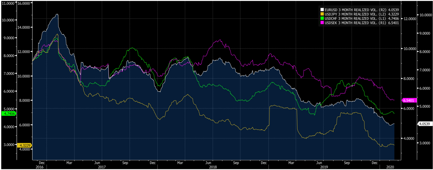
3 Month Realised Volatility for Selected Currency Pairs, Source: Bloomberg

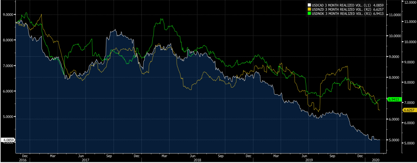
3 Month Realised Volatility for Selected Currency Pairs, Source: Bloomberg

The above graphs show the persistence of low volatility and the increasing downward force in FX volatility even through times where both equity and bond markets where experiencing high levels of volatility. That being said, it would be false to claim that FX volatility is dead as there have been a couple pairs that have been through periods of increasing volatility.

The most evident example is GBP. As it was exposed to tense geopolitical risks caused by Brexit, we can see GBP volatility outside of the downward volatility trend for certain periods of time, including last year.

GBP/USD 3 Month Historical Volatility, Source: Bloomberg

Another example would be AUD/JPY, which is frequently classified as a “risk-on” pair due to AUD’s China and commodities exposure. We have recently seen an uptick in AUD/JPY realised volatility as the Coronavirus-related news hit the market. In one month the 3 month historical volatility of AUD/JPY has increased from 7.6 to 8.2, clearly showing the “risk-on” nature of the pair.

AUD/JPY 3 Month Historical Volatility, Source: Bloomberg

As it can be seen from GBP/USD and AUD/JPY, volatility in FX markets is not dead. However, volatility seems to be less sensitive to non-geopolitical factors then it used to be. In the following sections our focus will be on potential factors that can explain such a behaviour.

Potential Reasons for Low FX Volatility

• Convergence of Inflation Expectations: inflation and inflation expectations are a key input of monetary policy, short-term and long-term interest rates, and many other key financial factors. From this perspective, we can say that divergences in inflation expectations could cause upward trends in FX volatility. High inflation generally tends to depreciate currencies; we can see this by looking at how inflation has lifted FX volatility in some EM currencies such as the Turkish Lira and the Argentinian Peso. Of course, high inflation is not the only reason why those currencies faced high volatility but obviously it was one of the causes of their experiences. Now, when speaking about G10 currencies we must specify an important characteristic: the fact that inflation expectations are not constant over time. As reported in the figure below, we can clearly see a downward trend in inflation expectations. If we were to observe a downward trend for a fraction of the G10 currencies only, we could then see an uplift of volatility. However, we see a persistent downward trend in all countries except the United Kingdom. As we explained in the previous section, we regard the GBP divergence as an idiosyncratic move caused by uncertainty about Brexit. So, except for the UK, there is a common pattern of inflation expectations among G10 economies, and we believe that this can be an important factor to explain why FX volatility is very low.

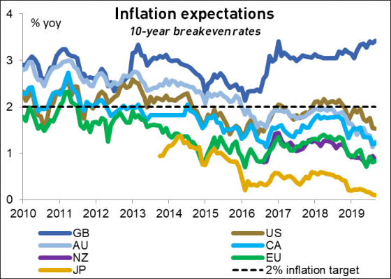
Source: Nasdaq

• Convergence of Monetary Policy: following our discussion about inflation expectations, it is quite intuitive to understand that the dominance of low inflation expectations across all developed markets makes central bankers face similar challenges. Indeed, it is clear that, with the prevailing trend of lower FX volatility, the odds that a major central bank hikes rates anytime soon seem to be very small. Overall, we can also see lower interest rate differentials between currencies as a consequence of globally lower interest rates, which have been in turn caused by globally low inflation expectations. From our point of view, lower interest rate differentials might have contributed to muted FX volatility.
• Limited Ammunition Causes Caution: as Europe and Japan are carrying out an experiment with negative interest rates, many monetary policymakers, including Jerome Powell of the FED, have ruled out negative rates from their side. This has an important implication: central banks think twice before cutting rates as they want to save room for a recession. As a result, the range of possible interest rates in the future is significantly reduced and we may observe lower FX volatility due to a lower range of future interest rate differentials.
• The Effort To Mitigate Uncertainty: we have started to see central bankers resorting to further forward guidance to fight uncertainty. The release of FOMC dot plots and the numerous times we heard former ECB governor Draghi assuring markets that he would not change rates for the foreseeable future are all factors decreasing the uncertainty of monetary policy which could, in turn, fuel FX volatility. In addition to making their thoughts about future monetary policy, we are seeing central bankers assuring markets that they would react to external shocks in a way that reduces market participants’ worries about the externalities of such events. This also is a factor which drives FX volatility down.

In a nutshell, we believe that the common low inflation expectation trend, convergence of monetary policy, stability of policy rates, caused by the fact that most central banks are currently operating with really low policy rates combined with too low appetite for negative interest rates, and the wide spread usage of forward guidance can be economic reasons for low FX volatility. That being said, we see political or external uncertainties, at a magnitude which cannot be mitigated by monetary policy, as potential reasons why volatility of AUD/JPY, over the past month, and GBP/USD, after the Brexit referendum, have been higher than their peers.

Is Carry Trade Dead?

While we have touched on FX volatility, it would also be meaningful to talk about how the new FX volatility environment could affect carry trade returns. First of all, it is important to understand that carry trades represent a significant share of FX trade flow and act as a force that ensures the uncovered interest rate parity holds in FX markets. The very reasons we presented as potential causes of low FX volatility (i.e. convergence of inflation and interest rates) can have effects on carry trade returns as well. Indeed, since the global financial crisis, we have seen carry trade returns stagnate considerably when compared to their pre-crisis performances. To demonstrate this, we are presenting two indices that are used to measure carry trade returns: FXCTEM8 (Bloomberg Cumulative FX Carry Trade Basket for 8 Emerging Market Currencies) and FXCTG10 (Bloomberg Cumulative FX Carry Trade Basket for G10 Currencies). Both indices represent the carry trade returns computed from their underlying currency baskets and they stated in values representing cumulative returns since their inception, so they were normalized to 100 in 1999.

Bloomberg Cumulative FX Carry Trade Basket for 8 Emerging Market Currencies, Source: Bloomberg

Bloomberg Cumulative FX Carry Trade Basket for 8 Emerging Market Currencies, Source: Bloomberg

Having seen the stagnation of carry trade returns and having talked about lower FX volatility, we thought about a potential relationship between carry trade returns and FX volatility. To test such relation on a very high level, we regressed J.P. Morgan Global FX Volatility Index on Bloomberg Cumulative Carry Trade Return for G10 Currencies Basket.

Y=J.P. Morgan Global FX Volatility Index; X= Bloomberg Cumulative FX Carry Return Basket for G10 Currencies, Source: Bloomberg

The results of our analysis point out a possible partial relationship between the two indexes. Consequently, we argue that carry trade returns and FX volatility are affected by common elements: this could explain the partial relationship shown by our regression and we believe that this argument makes sense from an economic standpoint as well. Due to various reasons, such as lower interest rate differentials, carry trade returns might be correlated with FX volatility. However, we think that extending the argument to an extent that says carry trade returns have a meaningful impact on FX volatility is hard with the results of the simple linear regression analysis we did.

Notice that a much richer statistical analysis would be required to assess the existence and the true extent of the relationship between FX volatility and carry trade returns. Even though that is not the purpose of this article, we provided a small but interesting hint, which may be more thoughtfully discussed in a future article.

Macroeconomic Factors and the EUR/USD Exchange Ratio

In this section, focusing our attention on the EUR/USD currency pair, we are going to investigate whether some macroeconomic factors have a significant effect on the volatility of the exchange ratio. Generally speaking, it is well known that asset price movements fail to be identically and independently distributed, thus implying the existence of clusters in their higher order moments. More specifically, large changes in values tend to be followed by large changes, and small changes tend to be followed by small changes. Volatility clustering may play a role in the explanation of the all-time low volatility of the EUR/USD exchange ratio and, consequently, requires us to base our investigation on a class of models that are well able to capture the departure of asset price changes from IID-ness: the ARCH-GARCH models.

The explanatory variables considered in this study are the inflation differential between the United States and the Euro Area (CPI), the percentage change in the monetary base of the United States (MONEY) and the differential between the 10-year Treasury and German Bund yields (SPREAD). CPI was computed as the squared monthly difference between the US Consumer Price Index and the Euro Area Harmonized Index of Consumer Prices, while SPREAD was measured as the squared difference between the 10-year Treasury yield and the corresponding Bund yield. All data are monthly spaced and refer to a period of 240 months from January 2000 to December 2019. Various sources were used to collect data including the Board of Governors of the Federal Reserve System, Eurostat and the OECD.

As a first step of our analysis, we checked the stationarity of the data through the classical Augmented Dickey-Fueller (ADF) test, whose results are shown below. Differently from CPI and MONEY, both EUR/USD and SPREAD are not stationary at level but are stationary when differenced once and, therefore, contain a unit root. Also, in order for our results not to be affected by their different scales and units of measurement, we standardised all the variables before proceeding with the estimation of a conditional mean model.

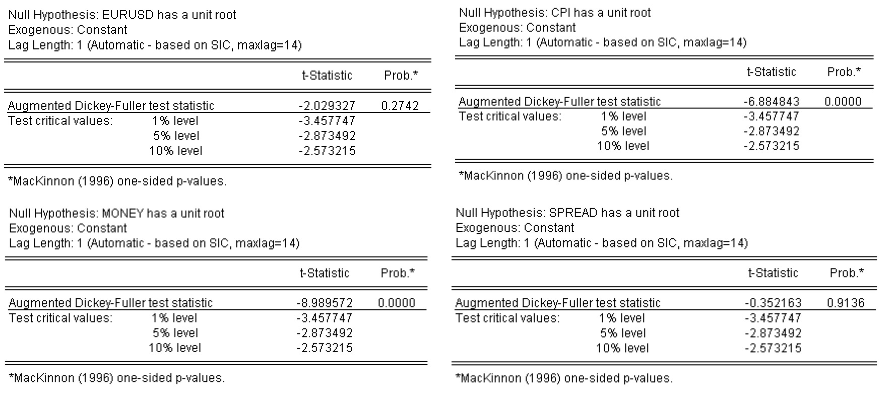
Augmented Dickey-Fueller Test at Level for Select Variables

The second step of our analysis was the estimation of a conditional mean model for EUR/USD, which was then fed into the GARCH model. In order to assess its best specification, we evaluated different models by minimising three of the most important Information Criteria: Akaike, Schwarz-Bayesian and Hannan-Quinn. As a result, we ended up selecting a MA(1) process, consistent with both the SBIC and HQ information criteria.

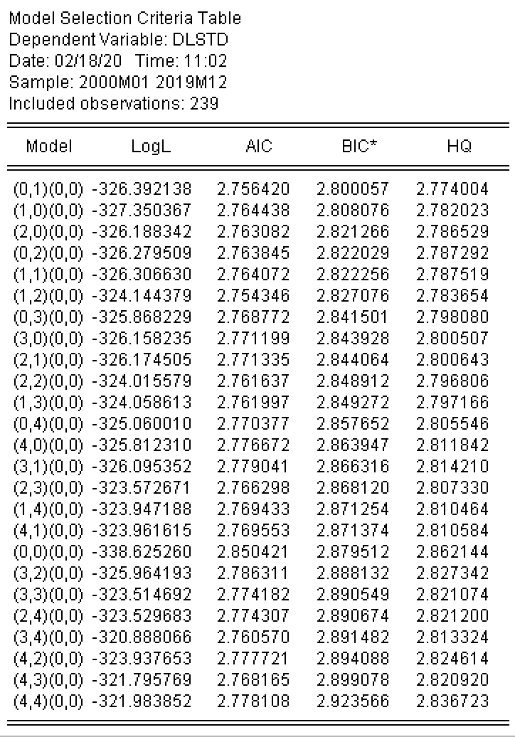
ARMA Criteria Table for EUR/USD

Therefore, the conditional mean model we selected is:

Where is the log of the EUR/USD exchange ratio in first difference and are the parameters of the model. As the focus of the analysis it to assess the effect of the macroeconomic factors on the EUR/USD volatility, there are no exogenous variables in the conditional mean equation.

Among the possible specifications of the conditional heteroskedasticity, we opted for a GARCH(1,1) which, as commonly acknowledged, is a rather simple model that can be shown to be equivalent to a much more richly parameterised ARCH model. Also, we added the macroeconomic factors into the equation, trying to evaluate whether they have a significant explanatory power for the conditional variance of the EUR/USD exchange ratio. As a result, we estimated the following equation:

Where is the variance of the residuals of the conditional mean model, is the constant, are the coefficients of the ARCH and GARCH terms and the macroeconomic factors, is the previous period conditional variance, is the previous period squared residual of the conditional mean model, and is the error term.

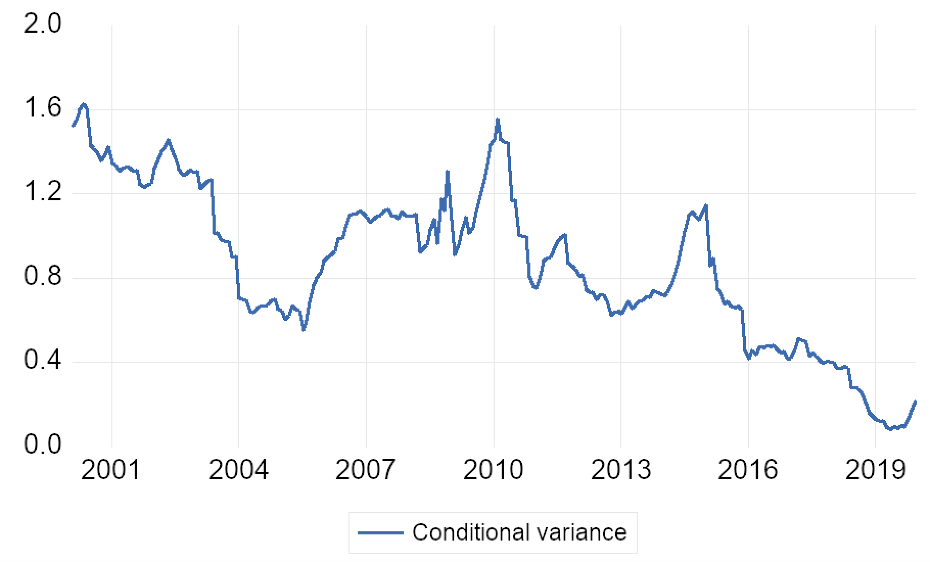
GARCH Variance Graph

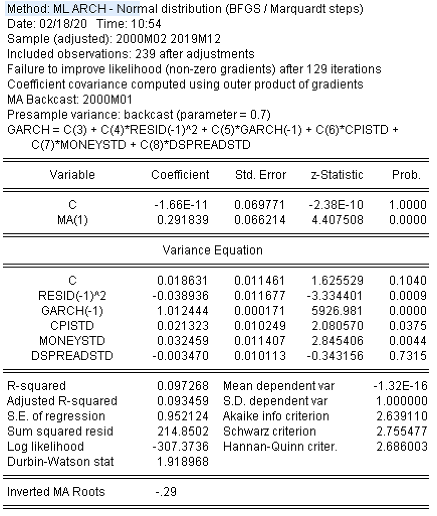
Results of GARCH(1,1)

As reported in the above figure, the coefficients of the ARCH and GARCH terms are significant at less than 1% confidence level. Under a normal distribution assumption, the model shows that both previous news and volatility influence current volatility. Consequently, as expected, the volatility of the EUR/USD exchange ratio seems to be affected by its own shocks. In addition, the coefficients of both CPI and MONEY are significant at the 5% confidence level, thus suggesting that the inflation differential and the money supply provided by the FED have an impact on the volatility of the Euro to US Dollar exchange rate. The coefficient of SPREAD is not significant and leads us to conclude that the spread between the 10-year Treasury and German Bund yields has no meaningful effect on the volatility of the currency pair.

The sign of the coefficient of CPI is consistent with our expectations. As we can anticipate a larger dispersion of inflation rates to be associated with a larger distance between them, CPI, which should be representative of the differential in the inflation rates of the United States and the Euro Area, was predicted to be positively related to the volatility of the EUR/USD exchange ratio. Conversely, the sign of the coefficient of MONEY is somehow different from the negative relationship you would expect between monetary stance, as measured by the change in monetary base, and exchange ratio volatility. A positive change in the monetary base is evidence of a more expansionary monetary policy which, as described in the previous section, should in turn lead to a lower volatility. A possible explanation for the result we obtained lies in the observation of the fact that the period characterised by the steepest declines in EUR/USD variability (i.e. from 2015 to 2019) is also the period in which the monetary base in the United States was stagnant or, better, slightly declining, thus leading to negative values for our MONEY variable.

Conclusion

The low volatility levels prevailing in FX are the culmination of a multi-year trend towards quieter currency markets. As extensively discussed, such behaviour is largely caused by easier monetary policies that followed the global financial crisis, spread across both developed and emerging economies, and still characterise the latest decisions of the vast majority of central banks. This theoretical reasoning seems to be supported by empirical evidence which, at least for the Euro/US Dollar currency pair, points out a significant relationship between the exchange rate volatility and some monetary policy-related macroeconomic factors, such as inflation differentials and money supply.

As a hawkisher behaviour of central banks is highly unlikely, unless economic growth and inflation unexpectedly peak up, we can forecast the declining FX volatility trend to continue in the near future. Two consequences transpire: buying currency options is relatively cheap and price swings are to be found in some non-traditional, more volatile currency pairs. Focusing on the first consequence, there are cases, such as the EUR/USD, in which realised volatility has already climbed above implied volatility, thus creating an edge to option-buyers and, generally speaking, whoever needs to hedge an exchange ratio risk. Secondly, as mentioned before, profitable opportunities may arise in specific currency markets: following the Brexit referendum, Sterling has become a relatively volatile currency, a trend that may be exacerbated by the approaching end of the transition period deadline; the AUD/JPY is a “risk-on” currency pair which might suffer from the full understanding of the Coronavirus outbreak; Eastern European currencies are increasingly characterised by diverging monetary stances, thus increasing their volatility; lastly, Asian currencies are already moving in response to Coronavirus-related news, a behaviour which is going to last until the extent of the economic damage caused by the outbreak is entirely priced into the markets.