The Mechanics of Commodity Swaps (BSIC x Dare)

Download PDF

Introduction

Commodity Swaps are a widely used instrument for hedging and speculation in the commodities markets. Like other swaps, they are an OTC instrument where two counterparties agree on exchanging some cashflows based on the trend of an underlying security (most often oil, but also other commodities like metals and grains). They usually anchor themselves on an index, and involve a floating and a fixed payment, where the fixed payer (or floating receiver) agrees to pay a fixed amount at specified terms (monthly, quarterly etc.) and receives instead a cashflow based on the average trend of the underlying commodity/index from the counterparty, whose obligations are the opposite.

They are used by a variety of different market participants, ranging from production companies, to consumers, to pure speculators of the sector, wishing to gain a particular exposure with a tailor-made contract.

History of the Product

Commodity Swaps are one of the oldest commodity derivatives present in the financial markets. Around since the mid 1970s (with the first ever oil swap established by Chase in 1986), are mainly used in industries where demand and supply dynamics tend to face heightened volatility, primarily the energy and agricultural market.

With the earliest instances of futures contracts on commodities being dated as far back as 2000 B.C. in Mesopotamia, the first ever regulated derivatives exchange still operating today is the Chicago Board of Trade (CBOT), opened in 1848 and saw the biggest expansion of its traded securities in the early-mid 70s, when, coincidentally with the collapse of the Bretton Woods Agreements, the advent of computational power and the advancements made in derivatives pricing by Black and Scholes. Since then, and up to the great revolution in regulatory laws post the 2008 crisis, derivatives contracts saw a huge expansion, particularly in the agricultural sector, due to the highly volatile nature of the market.

Definition and Key Features

A commodity swap is a legally binding agreement that guarantees a fixed price level. In this arrangement, one party commits to paying a ‘fixed index rate,’ while the other agrees to receive this fixed rate and, in turn, pays the ‘floating rate’ determined by the monthly average movement of the same underlying. Notably, the swap doesn’t affect the underlying sale or purchase transaction, which may involve another institution. The sole movement of funds involves a net transfer of payments between the two parties on predefined dates. However, with oil swaps, there is an option to link the swap with a specific physical cargo, with cash flows calculated based on an agreed notional amount, whether or not the cargo is actually delivered.

For instance, if the monthly average price falls below the strike, a shipping company can procure its fuel at a more favourable market price. Conversely, if the monthly average cost surpasses the strike, an oil company compensates the shipping company for the excess above the rate. An oil cap, for instance, fixes the shipping company’s bunker fuel costs at a maximum level, providing financial stability in a volatile market.

There are a couple of notable features that make it a versatile financial instrument. Firstly, it offers insurance protection, enabling counterparties to secure a fixed rate for purchasing or selling a predetermined quantity of oil or oil products over a specific time frame. Notably, no premium is required for this benefit. Furthermore, oil swaps present the option for cash or physical settlement, where typically, only the index-linked cash flows are exchanged, leaving the notional cargo quantity untouched. However, parties can arrange for physical settlement in advance if mutually agreed. Additionally, oil swaps facilitate funding optimization by allowing counterparties to work with institutions offering the most favourable prices for the underlying oil transactions, effectively decoupling the swap negotiations from these core dealings. It’s imperative to carefully evaluate the credit risk associated with both counterparties, as each party assumes the other’s credit risk. Oil swaps are typically zero-premium instruments, necessitating a credit line, but in some cases, counterparties may need to collateralize the swap with cash, through means such as a deposit or a variable letter of credit. These features collectively make oil swaps a powerful tool for risk management and price certainty.

Hedging – Futures vs Swaps

When it comes to hedging commodity exposure, there are distinct differences between utilizing commodity futures contracts and commodity swaps. Commodity swaps provide a more personalized approach, giving counterparties the opportunity to secure tailored insurance protection without the burden of a premium. This flexibility also enables them to optimize their funding by engaging in transactions where the most favourable prices are accessible. However, it’s important to note that commodity swaps come with their share of considerations, including the need for credit risk assessment and the potential for collateral requirements.

On the other hand, commodity futures contracts serve as more standardized and easily accessible mean of hedging. They provide a straightforward way to protect against commodity price fluctuations. However, they lack the level of customization found in swaps, which could limit their suitability for certain situations. Furthermore, commodity futures contracts often entail higher transaction costs due to initial margin requirements and the need for daily mark-to-market settlements.

Use Cases

As already discussed, commodity swaps are usually used for hedging by large corporations that wish to have more predictable cash flows in their cost of inputs or in the revenues coming from their outputs. In such a framework, we normally see the consumer paying the swap (i.e., paying fixed) and thus hedging on possibly rising costs for their inputs (a classic example of this would be an airline hedging the price of fuel or crude oil), whereas producers tend to receive the swap, putting a floor to a possible decrease in the price of the commodity.

To build up on this intuition, we propose a “textbook” example of hedging through commodity swaps:

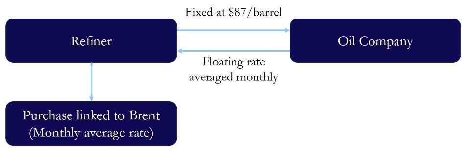
A prominent US oil refiner is concerned about another potential increase in Brent crude oil prices, due to the escalating geopolitical uncertainty and seeks to hedge around 120,000 barrels per month for a period of nine months starting November. To address this risk, the company intends to ‘pay the fixed and receive the floating’ rate, mirroring the underlying transaction. The company is content with entering the contract at the prevailing rates, and a major oil company offers a swap at $87.00 per barrel.

In this scenario the two parties would calculate and offset cashflows on pre-specified reset dates. For the sake of simplicity let’s say that in early December, when calculating the settlements for November, we observe the following rates:

Fixed: $87.00 per barrel

Monthly average: $90.00 per barrel

In that case the oil company would make a net payment of $3.00 per barrel to the refiner, totalling $360,000 for the initial 120,000 barrels. This effectively offsets the additional $3.00 per barrel that would have been incurred in the underlying market. Conversely, if the monthly average rate had been $85.00, the refiner would make the payment, resulting in a net cash settlement of $2.00 per barrel to the oil company.

Source: BSIC

Swaps however, just like other derivatives, also act as a powerful price discovery tool, for traders to set benchmarks on current prices in the spot market, while also allowing for lower transaction costs and overall increased market efficiency.

The latter also underscores the role of these derivatives as a means of speculation and as a way to express directional views on the trends and movements within the underlying markets. As a matter of fact, a second popular kind of commodity swap is the so-called “commodity-for-interest” swap, where, similarly to equity swaps, one leg pays the returns associated to a certain underlying commodity, and the other pays a floating interest rate (e.g., SOFR) or a predefined fixed rate. This type of contract enables counterparties to take on a directional exposure to anticipated returns of a specific commodity, and thanks to the cash-settled nature of the agreement, it eliminates the need for unnecessary costs associated with a physical delivery of the product.

Pricing

The most common way to think about commodity swaps is as being very similar to a fixed-for-floating interest rate swap, and a useful abstraction to build on this from a pricing perspective would be to imagine it as a series of forward contracts, just like IRSs are often associated to a bundle of FRAs (Forward Rate Agreements). However, a few additional elements typical for Commodity Swaps should be considered, the most notable ones being:

• Cost of Hedging
• Institutional structure of the commodity
• Liquidity of the underlying and its seasonality
• Credit risk

We can describe the pricing of a commodity swap simply by using the futures’ term structure of our underlying commodity to price the floating leg at origination, and then we can find the fixed rate in the following fashion:

We start by imposing the value of the contract to be 0 at inception, that is:

Where is the forward price at time with delivery at is price paid on the fixed leg and is the relative discount factor.

This is also equivalent to saying that the present value of all our future payments ought to be 0:

It follows that, immediately after origination, one can value the swap simply as or vice versa, depending on what side of the trade one has picked. This is because these swaps are linear contracts that involve no optionality.

In order to choose the appropriate forward prices/discount factors, dealers tend to look at market prices in the term structure and price the swap accordingly. In some instances, however, market prices tend not to be present or are highly unreliable. For instance, some commodities like grains or cattle, do not have futures contract expiring in every month of the year, but can display irregular patterns, which are often connected to the cycles of the underlying:

Term Structure of Lean Hog Futures as of Nov. 4^th

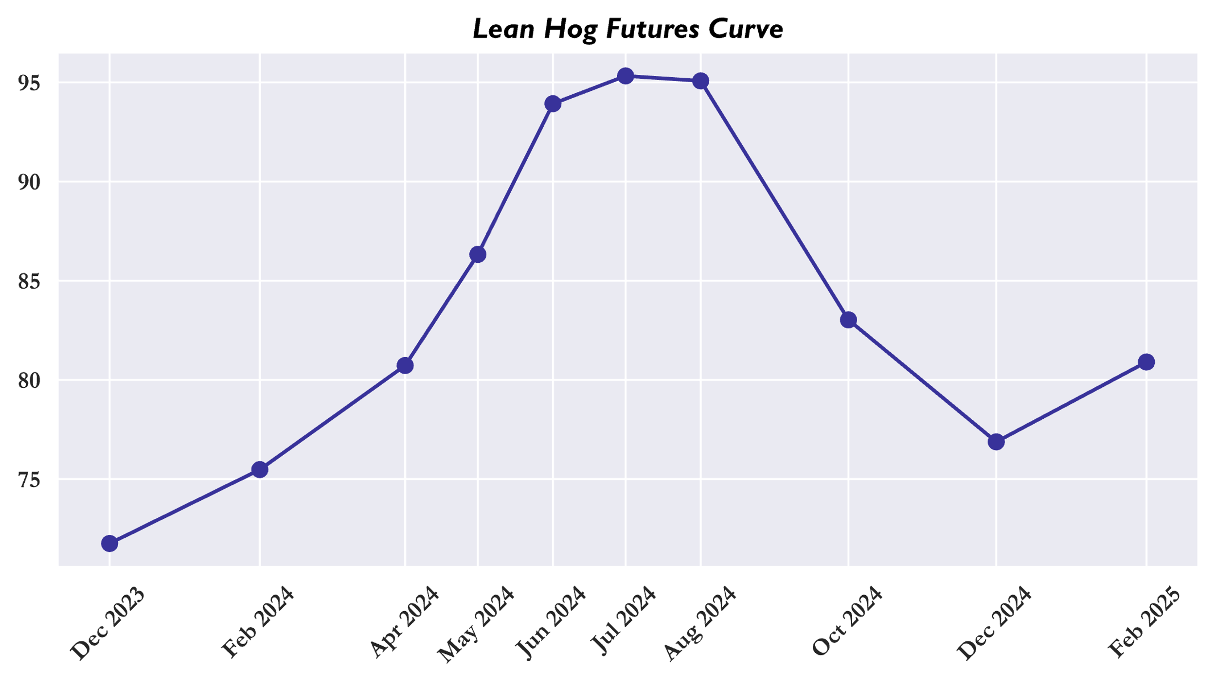
Source: OpenBB, BSIC

Similarly, in some specific contracts with longer maturities, like 5+ years, data from the market might be scarce or unreliable, as often the most traded section of the curve is the front end, with the back end often being crowded only by a few players, mainly big producers hedging their exposures. In such cases, modelling the forward curve might be necessary to model the fair value of the commodity far into the future and thus pricing longer maturity contracts.

Over the years, financial literature has proposed variety of possible quantitative models for such problems, which rely on one pivotal concept: “The scarcer the resource, the higher the volatility”. We can model forward curve changes, generally speaking, as translations (i.e., parallel shifts) and rotations (although some models also consider “twists” and seasonality).

For the sake of completeness, we will mention two of the more relevant models, although a more thorough analysis of their features, is outside the scope of this article:

Heath-Jarrow-Morton Model

The HJM model proposes the following two factors to explain the change in forward prices:

Where are centred and possibly correlated shocks, describes the term structure of futures prices drift and scales with the volatility. Note that we assume the “Samuelson effect”, which considers volatility a decaying factor of time to maturity, given mean-reversion.

Exponential Two and Three-factor Model

A special case of the abovementioned HJM model, in the exponential variation volatility terms are chosen to account for level and slope changes:

Note that the rotation factor, decays with time to maturity, whereas the shift factor is constant: If we also incorporate the twist, we have:

and

The Futurization of Swaps

In 2012, the Intercontinental Exchange (ICE) announced plans to transition all cleared OTC products listed on ICE’s OTC energy market to futures contracts. The move from swaps to futures was particularly impacted by Title VII of the Dodd-Frank Act, which sought to lower the levels of risk inherent to such transactions.

The new clearing mandates guaranteed that any financial losses arising from a defaulting counterparty are borne by sizable, autonomous institutions. This lessens the systemic risk associated with OTC derivatives trading and fosters greater market stability.

Trading shops can take advantage of the increased liquidity and transparency of futures markets to arbitrage between swaps and futures contracts. For example, a trader might buy a swap contract and then sell an offsetting futures contract on an exchange. If the price of the underlying asset moves in favour of the trader, they will make a profit on the futures contract and be able to offset any losses on the swap.

Developing an Edge – Trading

As swap products are not standardised in the same way as futures, their price is more open to speculation. For oil derivatives, the following products have standard pricing formulas for swap contracts:

• Brent Swaps
• Dubai Swaps
• Low Sulphur Gas Oil (LSGO/Ice Gas) Swaps
• Heating Oil Future Swaps
• RBOB Swaps
• WTI Swaps

The above products are priced based on a formula of the current futures value which also determines the settlement value at roll-off. For the swap contract of any given month, the price is determined by the arithmetic average of two forward month future prices which is heavily weighted to the first forward month.

All products with a standardised swap contract share a similar calculation strategy which varies slightly depending on product and month. This formula is also used to calculate the futures equivalent position of a swap contract as all risk is associated with the volatility of the front-month futures equivalent of these swap contracts.

For all other products – such 3.5% Fuel Oil Barges, Jet fuel etc. – there exist no standardised pricing formulae for swap contracts since the price offered is semi-subjective and opaque. In this case, a trader’s edge lies in their ability to best estimate the true value of the non-standardised product.

References

[1] Abumustafa, Naser I. “Hybrid securities and commodity swaps.” 12 Dec. 2006.

[2] Taylor, Francesca. Mastering the Commodities Markets. PEARSON, 2013.