“Well, CAN WE PREDICT?”: Backtesting Trading Strategies on Prediction Markets’ Cryptocurrency Contracts

Download PDF

Introduction/Recap:  

This article is intended to be a continuation of the previous “Well, CAN THEY PREDICT?” article which was focused upon developing methodology to price Kalshi weekly prediction contract probabilities of being in-the-money (specifically those functioning as a BTC digital option) using a risk-neutral framework upon stochastic processes. For more information regarding the mechanics of these digital contracts, it’s highly advised to read the opening remarks in the previous article.

Ultimately, we chose to use both Geometric Brownian Motion (GBM) with stochastic volatility on a RiskMetrics basis (volatility updates for each path at each timestep according to a RiskMetrics approach) as well as Merton’s Jump Diffusion. Additionally, we used the implied volatility of vanilla options on cryptocurrency exchanges to extract a risk-neutral probability density function which was then compared to the probabilities of each prediction contract. Both GBM with stochastic volatility and Merton’s Jump Diffusion models were within striking distance of the probabilities observed at a particular snapshot in time (right after the contracts opened); however, the IV-based approach proved to provide depressed levels of probabilities at each strike. Nonetheless, the utility of the IV-based approach on Kalshi contracts is negligible due to the differences in expiries, meaning that the probabilities of being in the money do not reflect the same event. For this reason, we’ve decided to omit this approach from the current article.

Now, we’re putting this idea (somewhat) into practice: in this article, we aim to test the predictive power of our GBM models by backtesting a trading strategy dependent on such ability. First, details about our approach will be explored along with their respective nuances. Naturally, our results will then be presented and discussed. Then and only then will we know if it’s feasible to suggest that these market participants may be mispricing these contracts according to the assumption of stochastic price action.

The Main Idea: 

Our approach consists of springboarding off the stochastic process rationale we established in the previous article: instead of using snapshots, we use dynamically changing stochastic processes where parameters are frequently adjusted to reflect price action and volatility throughout the maturity of the contract. By doing so, we hope to spot dislocations between our models’ expectations for being in the money as opposed to Polymarket’s participants’. Lastly, we use these dislocations as signals to buy or sell these prediction contracts in addition to how to size the position. All these details will be further explained in depth within the coming paragraphs.

Finding The Contracts: 

Initially, our goal was to leverage the same Kalshi contracts we identified in the previous article. This would mean weekly contracts with standard European option mechanics: quite straightforward. Moreover, these contracts had a plethora of strikes and had more than one year of tick data. Unfortunately, there was one key component these Kalshi contracts just didn’t have: liquidity. Naturally, this means that if any divergences had been present in the first place, they wouldn’t be tradeable due to abhorrently high bid-ask spreads on the orderbook. For instance, there are quite frequent instances at which most strikes have a 1-100 bid-ask spread. Additionally, from a computational perspective, running a 50,000 path GBM at each tick puts considerable stress on most hardware, including ours. So, we pivoted: we decided to grab Polymarket’s hourly data on a similar (but not identical) weekly Bitcoin contract at various strikes.

The key difference between Polymarket’s contracts and Kalshi’s is that most of the strikes have ranges; in other words, the probability of being in the money for each contract needs to be bounded. For instance, if the strike is stated to be “92-94k”, being in-the-money would mean that, at expiry, the price of BTC would lie within that range. Lastly, you have the unbounded probabilities in each direction. An example of such contracts could be bidirectional strikes of “>102k” and “<92k.” Fortunately, from a risk-neutral perspective, our initial assumptions for the stochastic process still hold when trying to estimate future probabilities, as these contracts can simply be seen as combinations of vanilla call-put options which can be used to replicate the same payoff profile (iron condor for “range” contracts, standard calls/puts for the “unbounded” contracts). And, most importantly, the Polymarket contracts possess significantly higher liquidity, albeit still not deep enough to support sizeable trades without moving markets.

The biggest tradeoff, however, is the time series itself: we no longer have access tick data when using Polymarket, and the length of the time series is reduced to 6 weekly contracts. At this point, it becomes important to stress that this article is only trying to achieve proof of concept. With such data constrictions on a very time-sensitive strategy, we simply wish to prove the feasibility of the formerly mentioned hypothesis.

Application of Methodology: 

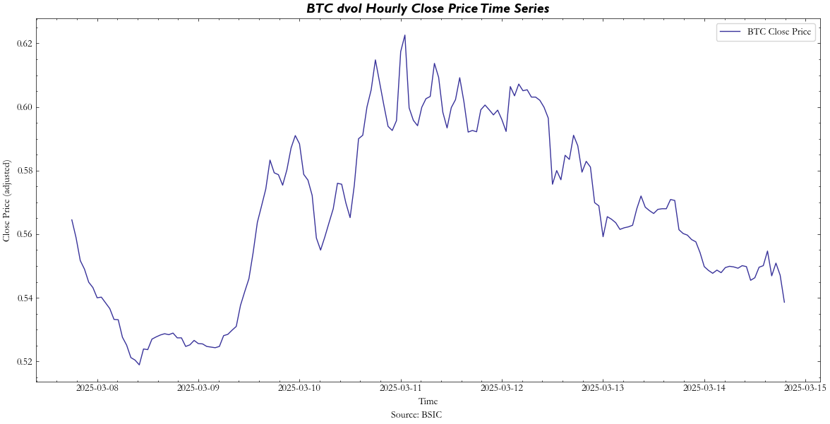
Now, the fun stuff. Once again, to get a better idea of the concepts we’re about to go into, please refer to the previous article. First, let’s briefly cover how we approached each of the relevant parameters for both the Jump and GBM Models. For the diffusion/  term, we had initially chosen RiskMetrics-based historical volatility due to its simplicity of calculation. However, in order to increase robustness, we now use Deribit’s Volatility Index (DVOL), which is an expected 30-day annualized implied volatility index derived from Deribit BTC options. The intuition for its usage as a diffusion term is that the forward-looking and dynamic nature of such an index will give a much more dependable indicator for volatility within 7 days as opposed to relying on a RiskMetrics model where you’re subject to determining the best for your half-life. Additionally, with 9 out of 10 BTC options being traded on Deribit’s exchange, we assume that the exchange is the most liquid and hence reliable when it comes to providing IV data:

Next, we consider our drift term, . The initial plan was to use the same implied funding rate from the basis of BTC 3-month delivery futures that we used in the initial article. The reason we thought this would be more apt for the sake of our stochastic processes is similar to the reasoning for the implied volatility: a lot more dynamic, and it directly addresses the carry costs and risk premia of holding our underlying asset, Bitcoin, which would keep it more consistent with the risk-neutral framework. Unfortunately, finding time series data for such a metric proved to be quite difficult and wouldn’t be feasible to find within our given timeframe. Ultimately, we decided to use the risk-free rate with our proxy being the 1-month US T-Bill rate.

For our jump parameters (, jump mean, jump standard deviation), we decided to use a rolling window of 7 days on which we calculate how many hourly fluctuations exceed two standard deviations based on our RiskMetrics-adjusted historical volatility () and then we calculate our statistical moments based off of the datapoints which fulfill this requirement.

Lastly, our stochastic volatility is updated upon each path according to a RiskMetrics approach where our   is set to a value of 0.998 (approx. 7 days)

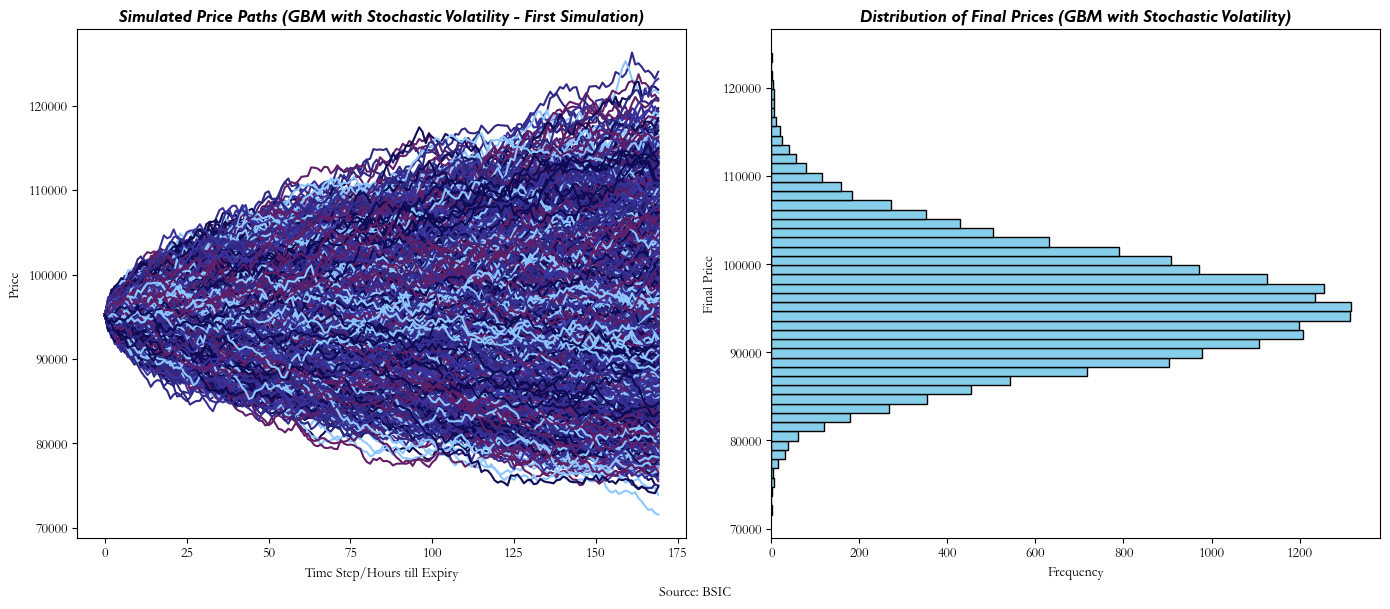
Using all these parameters, our Stochastic Volatility Model ends up looking something like this at any given hour until expiry:

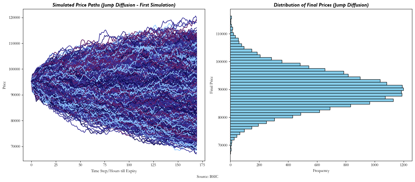
And, similarly, our Jump Diffusion will look something like this:

Now, by using the final prices distribution, we can deduce what our models’ probability estimations are, regardless of whether they are ‘range’ or ‘unbounded’ strike contracts. 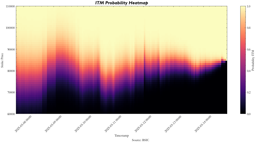But in order to understand how the probability of being in the money for each particular contract changes as time progresses, we need to create a new stochastic process at each hour, updating each of the aforementioned parameters (, , , etc.) to see what the probabilities at each timestamp would be. Intuitively, this also means that at each hour, we also reduce the number of steps to reflect how many are left till expiry. We can show this behavior through a heatmap, which represents how our probabilities for a given strike (and contract) move through time:

After aggregating all the probabilities for a given contract throughout maturity, they look something like this:

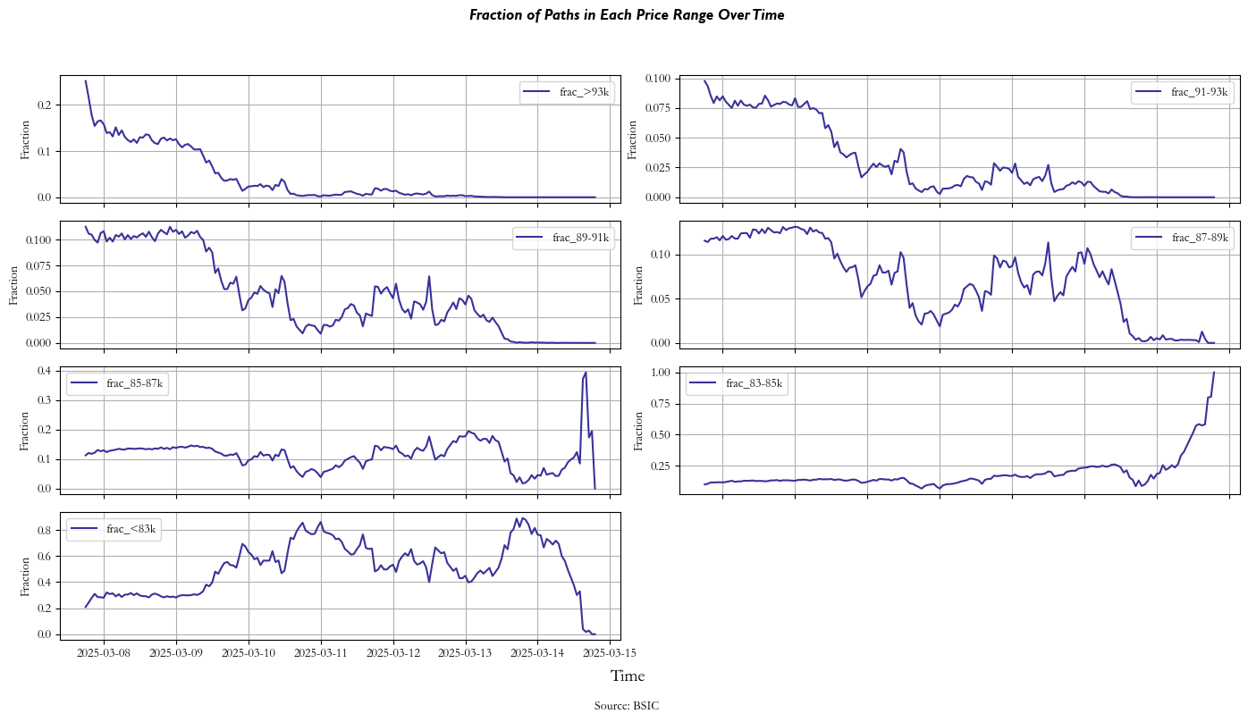
Finally, we get to the comparison part of the article. After the probabilities for each strike and contract are calculated throughout maturity, we can calculate their dislocations by simply taking their difference through the time series:

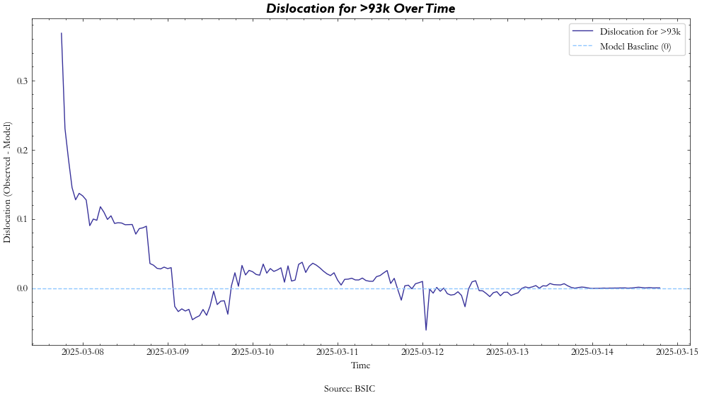
As shown in the figure, the process of the contract starts with high illiquidity and a large dislocation but starts to quickly show behaviors of mean reversion around our model. This is a behavior we observe across most contracts at most strikes.

Now, the rationale for our strategy was to leverage the times at which these dislocations were large and rely on them reverting to our model’s prediction. For instance, go short with a positive dislocation, long with a negative dislocation.

Our first intuition was to apply an expanding sigmoid function going from –1 to 1 to our dislocations and hold a sample portfolio proportional to the inverse of the weight given by the sigmoid function’s output. We attempted this with the function:

Where is the normalized time series of dislocations. However, we ran into two main issues using this as our backtesting logic inherent in our time series data: first, we had overlaps between the expiration dates of some contracts and the releases of the subsequent ones, and second, the price ranges offered by the market weren’t consistent from one contract to the next. Due to time constraints of our study, the scope of our research, and because we couldn’t find a logical way to aggregate dislocation behavior across strikes and overlapping timeseries without making various preposterous assumptions, we decided to simply our trading logic—which, yes, we will optimize at another time:

1. We bootstrap 50 data points from each contract to get a standard deviation of dislocations that we will use as a benchmark.
2. Then, we implement a simple rule: if the contract price is 1 standard deviation above the implied price given by our model, we go short 1 unit until the price reverts to just 0.1 standard deviations above the implied price after which we exit our position; vice versa.
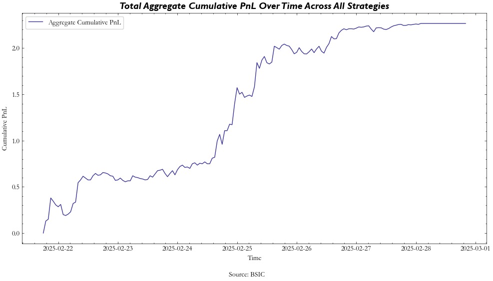
3. We then implement the strategy across all strikes with the same expiration date and aggregate the cumulative returns to get our PnL.

This also helps us get a more robust idea of performance considering transaction costs, since continuous rebalancing (sigmoid outputs) incurs heavy transaction costs and requires a certain confidence in the available liquidity. Below is a sample of the aggregate returns and risk metrics.

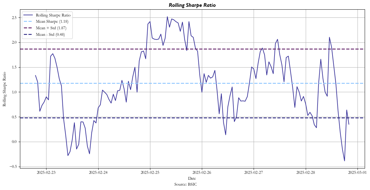
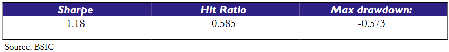
In addition to our Sharpe, we have a positive hit ratio (hourly in our case) of 0.585, telling us that our strategy makes winning trades over 58% of the time. Additionally, our strong max drawdown is not something to be overly concerned about as it is a byproduct of trading in unit increments — drawdowns in the beginning of the trading period will become an overly large part of the drawdown. Changing the trade sizing so that it is proportional to the portfolio should improve this metric greatly, but that is outside of the scope of the current article. Either way, we see smaller and smaller drawdowns as the time series progresses in our case.

Conclusion 

It’s safe to say that results proved to be quite promising with respect to our strategy. However, the most glaring issue with reproducing such a strategy in practice is the depth of the liquidity, or lack thereof. If a buy or sell order’s size is larger than 3 figures, most times, you’re immediately moving the spread. Still, if dislocations are large enough and we set higher bands to trade and account for this lack of liquidity, then this strategy may be profitable if you’re running a smaller account.

Another caveat is that our model gives us abnormally large movements in probabilities as we approach expiry. For instance, dislocations around 6 hours before expiry will experience a huge spike and then return to previous levels. This could potentially be attributed to less than optimal parameter selection. As mentioned previously, we’re using implied volatility from DVOL which is an expected 30-day annualized metric, but this means that the standard dynamics of options leads to an over-estimation of price swings in the final hours. Additionally, it could partially be due to a less-than-optimal drift parameter (RFR). Instead, an implied funding rate may result in higher predictive power due to its more robust nature as a metric with respect to the risk-neutral framework.

Once again, using more granular tick data would better inform our GBM and empower it to make more informed decisions throughout time. For a volatile asset such as BTC, this can become crucial to capture short-term shocks which have the potential to be extremely large.

In the future, if liquidity still proves to be quite small, replicating this strategy on various other crypto-related Polymarket contracts (Ethereum, Solana) with European-style resolutions could yield similar results and allow for larger size to enter the market, as long as the sizing of each trade accounts for that respective contract’s order book depth.