What works today might not work tomorrow: overview of a Systematic FX Strategy

Download PDF

Introduction

One of the main drivers of foreign exchange rates is the change in current and expected interest rates, influenced by central banks’ forward guidance and economic releases. In this article, we explore a paper by Nicolas Georges (2014) and implement a systematic FX strategy on G10 currencies, which trades based on changes in the expected path of interest rate differentials. In the first section, we explain the concepts behind the traditional FX carry strategy, providing some economic intuition on the existence of a risk premium. In the subsequent sections, we explore how the strategy distinguishes itself from the traditional carry trade, how the signal is constructed, and the data we use. Then, we backtest the strategy, providing some economic intuition on why it stopped performing after 2011. We finally conduct robustness checks and factor analysis to explain its returns.

FX Drivers and the Carry Trade

Currency valuations are mainly driven by three factors: changes in interest rates, which favor higher-yielding currencies; changes in inflation expectations, which depend on the macroeconomic cycle and the credibility of central banks; and changes in trade, which favor net exporters due to higher capital flows.

The interest rate differential between two countries gives rise to the classical carry trade: borrowing in a low-yielding currency and investing in a high-yielding currency. For a primer on FX carry trading, please refer to this article. The Uncovered Interest Rate Parity (UIP) condition states that the difference in interest rates between two countries will equal the relative change in the foreign exchange rate over the same period, therefore canceling out any profits of the FX carry strategy. However, the UIP does not hold in practice; the expected profits from a carry trade correspond to a risk premium. The central pricing equation states that the current price of an asset is equal to its expected payoff plus a risk premium, and it can be decomposed as follows:

In the above equation, represents the price of the asset, represents the payoff of the asset, represents the degree to which investors value consumption today over consumption in the future and represents the marginal utility function. The risk premium can be decomposed into three terms: the correlation between the payoff of the asset and the marginal utility, the volatility of the marginal utility, and the asset volatility.

This intuition can be applied to currencies as well and results in the forward rate being equal to the expected future spot rate plus a risk premium, which similarly, depends on the correlation between the marginal utility of consumers and the spot rate, the volatility of the marginal utility and the spot rate volatility. Since currencies exhibit a strong correlation to the wider economy and the marginal utility’s and spot rate’s volatilities can’t be 0, assuming they are not constant, we deduce that the risk premium should be non-negative. In general, investments in currencies that are mostly correlated with the wider economy (EMs) require a large and positive risk premium, while investments in currencies that act as a portfolio hedge may command a negative risk premium. Therefore, the future spot rate is not equal to the forward rate and the UIP doesn’t hold. [2]

Strategy Implementation and Signal Construction

The difference between this strategy and the classical FX carry trade is that it exploits movements in rate expectations, by systematically buying currencies whose rate expectations rise and selling the ones whose rate expectations fall. The strategy covers all the currencies of the G10 and can therefore be long and short any mix of high and low-yielding currencies, based on the interest rate expectations. It implements a simple signal (+1/-1) based on the simple moving average of the rate differential. Specifically, it goes long currency 2/short currency 1 when the yield is above the moving average and long currency 1/short currency 2 when the yield is below the moving average. As for the interest rate expectations, the paper uses as a proxy the 2Y FX Swaps rates.

The strategy is always rebalanced at the London close; if a significant move in yields is realized between the London and New York closes, a second rebalance is made at the latter. All currencies are converted to CCY/USD format, and the positions are computed in USD.

The signal for a specific currency CC1 is the sum of all the sub-signals CC1/CC2, CC1/CC3, CC1/CC4, and so on, for all the remaining currencies in the basket. To compute the signals, we follow this process:

• Initialize signal to 0 for each currency (AUD, CAD, …)
• For each country1, country2 in combinations (countries, 2)
  • Compute the current differential between country1 and country2
  • Compute the moving average (MA) of the differential over X days (the window)
  • Sub-signal (country1, country2) = (Differential – MA) / ABS(MA)
• Compute the percentile at 50% of the absolute values of all the sub-signals
• For each sub-signal, if the sub-signal is over the percentile
  • If country1 is not USD: signal(country1) += sign of sub-signal
  • If country2 is not USD: signal(country2) -= sign of sub-signal

To calculate the positions, we target a fixed Gross Total Exposure (defined as the absolute sum of all nominal positions), which we set to $1,000,000 in the backtest. We size the positions relative to each signal’s value, thus giving more weight to currencies that have strong signals in either direction.

Backtests

All the code for the backtester and further analysis can be found on this GitHub repository. As opposed to the paper, which calculates the signal and positions for each day subsequently, we vectorized everything to compute the signal and positions for all days at the start. We compute the P&L accounting for transaction costs, using the slippages for each currency provided by the paper.

We backtested the strategy from 2000 to 2020, using Python. We first implemented the strategy as described by the paper, using 2 days for the short-term signal, and 15 days for the long-term signal.

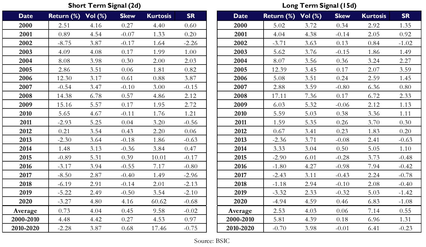
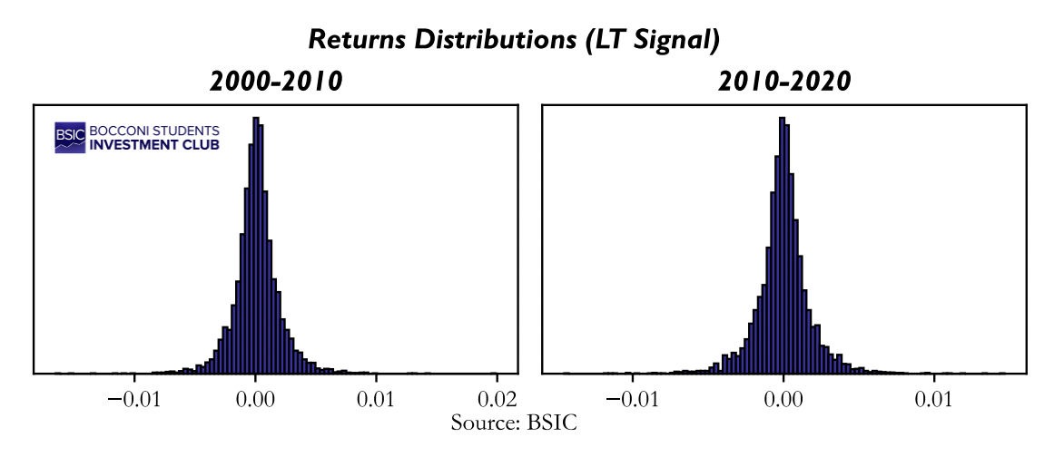
We immediately see a very interesting finding: the strategy performed fairly well up until 2011, after which returns started to decline. Looking at the return distributions, we find that they are positively skewed and present significant kurtosis (fat tails). This is to be expected due to the nature of FX prices, which are subject to jumps following Central Banks’ announcements and main economic releases.

But why did the strategy stop performing after 2011? We think it may be due to several factors.

First of all, 2010 marked the start of a period of extremely low interest rates across almost all G10 countries. Rather than harvesting differentials among DMs, investors were forced to shift more aggressively to EMs to get attractive returns. Secondly, the sovereign debt crisis in 2011, which started in Greece and spread to Spain, Portugal, and Ireland, sparked concerns among investors and led the DM’s currencies to be driven more by a “flight to safety” narrative, rather than by differentials. This hypothesis is supported also, for instance, by looking at the period between 2016 and 2018: with the Fed hiking and the other CBs on hold, differentials were moving in favor of the USD, but the currency kept depreciating regardless.

Robustness Checks

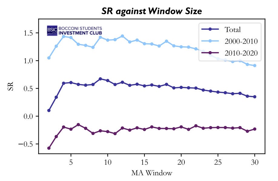
We conducted robustness checks for the strategy, computing SR as a function of the rolling mean window and changing the rebalancing frequency.

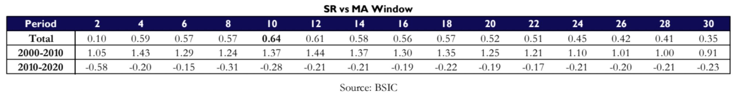
If we look at the two periods separately, the signal seems robust with respect to the MA window, both in 2000- 2010 and in 2010-2020. After removing the 2-day window (which leads to a too-unstable signal anyway), the SRs for the two periods have a standard deviation of 0.17 and 0.04, respectively. However, considering the wide (and consistent) spread in sharpes between the two periods, we conclude the strategy is not robust with respect to structural changes in the market.

Factor Analysis

We performed a factor analysis of the strategy against the main factors driving FX returns: carry, momentum, and value. The carry factor is computed by going long the higher-yielding currencies and short the lowest-yielding; the momentum factor is constructed by going long the best-performing pairs, and short the worst, based on past returns; value uses Purchasing Power Parity (PPP) between countries as a proxy of each currency’s cheapness/richness. Finally, we also added a market factor, constructed using a long-only, equally-weighted portfolio of the currencies covered by the strategy.

Due to the nature of jumps in FX, which make returns non-normally distributed, we opted for a Robust Linear Model (RLM), rather than a traditional OLS Regression. In the RLM, the function to minimize underweights outliers, which would “pollute” results in a normal OLS. Since the performance of the strategy differs significantly between the two time periods, we performed the factor analysis separately for 2000-2010, and 2010-2020. The regression is performed using monthly returns.

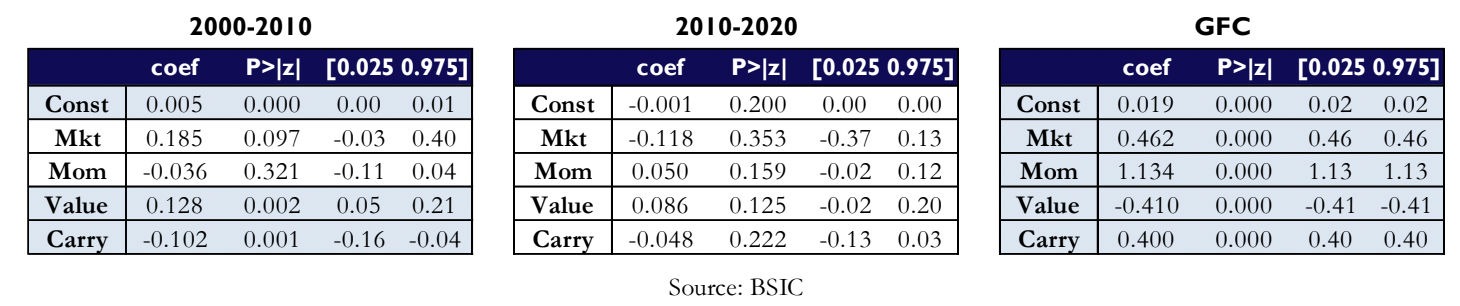
While, for the period between 2010 and 2020, none of the factors is statistically significant to explain the returns, we find that, between 2000 and 2010, value and carry seem to explain part of the variance. However, the factors to which the strategy is exposed are very volatile and subject to the timeframe one takes into consideration. For instance, if we look at the period between 2008 and 2009 (GFC), we find that the strategy was very long momentum, short value, long carry, and long the market, with every factor being statistically significant with a p-value < 0.001.

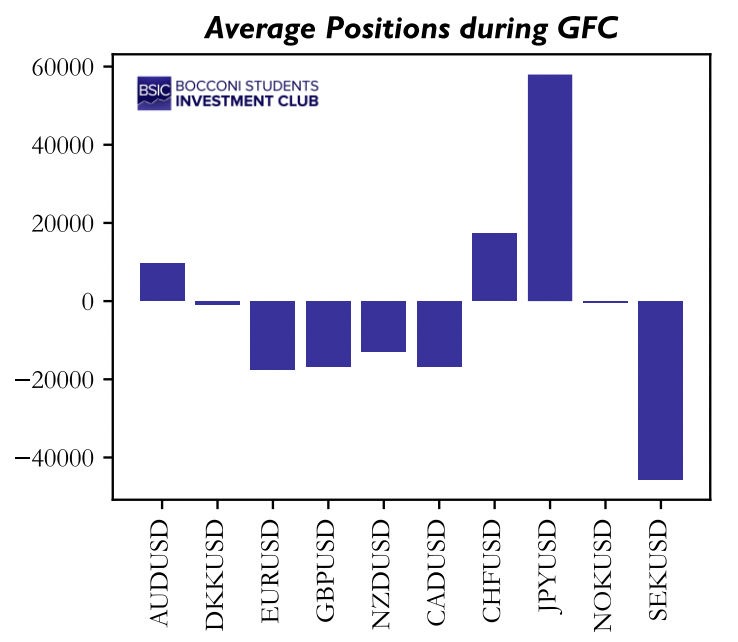
Plotting the average positions during the GFC confirms the results of the regression: the strategy was long the main safe haven currencies (CHF, JPY) and short European currencies (which were suffering due to spillover effects).

Next Steps and Conclusion

In this section, we are going to elaborate on how we think the strategy may be improved and what we tried while working on the article.

First, one could try to incorporate expected inflation in the differentials, to get a proxy of the future expected path of “real” rates. This has proven challenging due to several reasons: first, getting expected inflation data for smaller countries is more complicated, since they don’t have inflation swaps or TIPS-like securities, and if they have, yields are “polluted” by high liquidity and inflation risk premia. Furthermore, higher inflation surprises in DMs don’t have the same effect as in EMs: G10 Central Banks are credible and markets believe their capability to tame inflation, so the currency usually appreciates initially.

Then, to improve the signal, we applied an EWMA (Exponentially Weighted Moving Average) instead of a rolling mean, mixed short-term and long-term signals, and accounted for the heterogeneous volatility of differentials by constructing a rolling z-score. However, the improvements were marginal, with the drawback of adding more hyperparameters and thus more uncertainty to the model.

Finally, this strategy could be expanded to EM currencies. However, the way EM FX behaves is rather different from the way DM FX does: for instance, an upward revision in expected inflation would boost the currency in a DM, but will usually cause the EM currency to depreciate. This is because markets don’t usually believe in the EM CB’s capability to tame inflation and keep interest rates high for long enough while at the same time not damaging the economy.

In conclusion, we think that, although the strategy had a statistically significant edge before 2011, this does not hold anymore. It will underperform during periods of widespread low interest rates and periods of market distress, where flight to safety becomes the key driver in FX returns. Neither the robustness checks we performed nor the factor analysis, support the hypothesis that the strategy may start outperforming again in the future.

References

[1] ANANTA, a Systematic Quantitative FX Trading Strategy, by Nicolas Georges (2014)

[2] Foreign Exchange, Practical Asset Pricing and Macroeconomic Theory, by Adam S. Iqbal