Sink or Swim: A Primer on the Crude Shipping Market and Frontline

Download PDF

Executive Summary

On February 28th and in the subsequent days the first wave of headlines were released:

“Israel and the U.S. Strike Hundreds of Targets: Nuclear Sites and Missile Launchers Hit in the First Wave” – House of Commons Library. 

“IRGC Launches ‘Operation True Promise 4’: Hundreds of Missiles Target U.S. Bases in Qatar, UAE, and Bahrain” – Fars News Agency. 

“Iran State TV Confirms Khamenei ‘Martyred’ alongside Family Members; 40 Days of Mourning Declared” – Caspian News. 

In this article we offer a primer on shipping economics and conduct an analysis of the crude oil market, particularly with respect to Brent. We continue by examining the specific market dynamics which are being affected by the Iran-U.S. conflict, define implied probabilities around the duration and intensity of the conflict and attempt to model spot freight rate prices accordingly. This provides us with a baseline for analysing Frontline’s fleet portfolio, likely free cash flow and dividend yields; we outline both its bond-like and option-like behaviour. Finally, we propose an options overlay to ensure that in the event of material changes in the oil market our risk is measured.

Frontline [FRO: NYSE], despite the predictions of elevated crude prices and concerns regarding closure of the Strait of Hormuz, finished the Monday session 1.6% up, fading from a 5.32% opening jump from its Friday close. Tanker equities often open strong on the intuitive thesis ‘disruption = higher freight costs’. However, at present this event is becoming increasingly global rather than localised and the market is asking a different question: is this a freight-positive supply shock, or a macro-demand negative shock, or both? 

In a market where conflict is expected to persist, the risk of recession, demand destruction and policy response are all discounted and investors forced to de-rate many sectors which exhibit cyclical behavior. Additionally, the information available on the Strait status is scarce: reports describe closure and threats to attack transiting ships, while others write traffic may simply be slowing or restricted. 

It is important to underline that tanker equities are not a play on freight spot rates; rather, they are a bet on the sustainability and deliverability of the higher earnings. Even if spot rates rise, there are a multitude of items that one has to discount when trying to understand how revenue items convert to sustainable equity gain. Factors such as (i) operational factors (i.e. shipowners not sailing to war zones), (ii) war risk insurance and other routing adjustments that add costs and therefore reduce the effective supply of tonnage from shipowners, and (iii) any potential government interventions to try and manage upward moves in rates (by ordering emergency supplies or through diplomatic means in an attempt to prevent an OPEC+ response) obfuscate the relationship between equity value and freight rates.

Introduction on Global Shipping 

Before we can look at the specific structure of the crude markets, freight spot rates, and FRO, we need to understand the main characteristics of shipping. The world freight market is divided by different types of cargo, ship designs and routes. That said, the economics of shipping possess a similar characteristic: demand is derived rather than inductive. Demand for crude tankers is derived from the world’s consumption of oil products, and the imbalance of crude production and oil consumption locations. Oil is produced at those places on the Earth’s surface where geological conditions are favorable for extraction and is generally refined at those locations and centers which have adequate capital. 

The structure of freight is granular and dependent on numerous factors including basin level export volumes, refinery maintenance, port congestion, canal access, weather, sanctions compliance and terminal waiting time among other items. The ‘market’ consists of a mix of regional micro-markets that are linked imperfectly through vessel substitution and ballasting flows. As a result, the increased time it takes for information to diffuse across the market can drive prices away from market fundamentals.

In crude shipping, information is operational, dispersed, and often based on relationships. Chartering activity occurs through brokers; cargo fixtures are reported with delays; deviations, delays, insurance restrictions, and compliance decisions are often not immediately visible in public data. Furthermore, the structure of oil prices, especially a contango futures curve, can create demand for floating storage. This can temporarily turn transport vessels into storage assets and reduce the effective supply. In such situations, freight rates can rise, even when consumption remains the same. This fragmentation weakens the strict form of the Efficient Market Hypothesis in tanker equities and freight derivatives. Prices do not instantaneously incorporate all relevant operational information because that information is neither perfectly observable nor uniformly distributed. Therefore, arbitrage, whether between spot freight and tanker equities, freight futures (FFAs) and physical fixtures, or between regional route spreads, can persist. 

Conversely, the ‘constant’ nature of shipping demand is contrasted by highly constrained supply. In the short run fleet supply is nearly fixed. Ships already built must operate, and their marginal operating costs are relatively low compared to capital costs. Given the inelastic nature of supply in the short-term, small shifts in ton-mile demand can generate disproportionate movements in rates, and this convexity explains the extreme volatility characteristic of crude tanker markets.

It is important to underline that tankers are capital-intensive and highly specialized assets: a Very Large Crude Carrier (VLCC) cannot be easily converted to alternative use. When freight rates collapse, owners cannot quickly exit the industry. Supply persists despite losses, prolonging downturns. Conversely, during booms, investment surges. However, shipbuilding involves long lead times with an average delivery time of 2 or 3 years.

Tonne-Mile calculations are a key demand metric for analysis. They are calculated as the product of cargo volume transported (in metric tonnes) and the distance of voyage (in nautical miles) and is more accurate than volume alone:

This is why chokepoint disruptions have disproportionate impacts on VLCC freight rates: vessel supply is fixed in the short run, but effective demand (measured in tonne-miles) can rise dramatically when trade routes lengthen.

Spot freight rates in the VLCC market are quoted on the Baltic Exchange’s Tanker Route Assessments, expressed as Worldscales (WS) points. Worldscale is a tanker freight system established in 1969 that sets a flat rate per tonnage for each port-to-port route on a nominal benchmark voyage. The organization publishes a table of flat rates annually (in US dollars per metric tonne) for a standardized tanker voyage between thousands of port pairs. The calculations often assume a standard vessel of 75000 DWT, though VLCC rates are often separately benchmarked. In addition, it outlines a reference bunker price, standard port costs, and a fixed daily hire rate of $12, 000 per day. Actual rates are noted as a percentage of flare rates (WS=50 = 50%, WS 200 = 200%).

TCE is the industry-standard profitability metric, stripping out voyage-specific costs (port dues, bunker fuel, canal fees, war-risk insurance) to produce a comparable daily earnings figure.

At high freight rates, operators accelerate their vessels from typical slow-steaming speeds (approximately 10-11 knots) to maximum sea speed (approximately 14-15 knots for a laden VLCC). Speed has a cubic relationship with fuel consumption (the Admiralty Coefficient):

At 15 knots versus 11 knots, fuel consumption increases approximately 2.5-3x. At pre-crisis fuel prices, this would be economically irrational; at $250,000 per day freight, the incremental fuel cost is irrelevant relative to the faster revenue generation.

Secondhand Vessel Values and NAV

Ship values are the largest component of the NAV calculation in equity analysis for tanker companies. Secondhand vessel prices are set in private, bilateral markets where negotiations occur between a single buyer and seller and generally in accordance with prices quoted by shipbrokers such as Clarksons, Barrass and Baremer (Arrow) as well as others. The values of these secondhand vessels are a function of:

Newbuilding prices in VLCC sector are crucial as these form the ceiling for the replacement values of secondhand ship prices. If secondhand ship prices approach or breach the newbuilding prices, then owners will opt to build more ships thereby capping upward movement in prices. Similarly, the scrap prices act as the effective floor for the price determination and thereby compresses the trading band when freight rates are still firm. 

The terminal value of a tanker asset is its scrap value at the end of its economic life, typically when it is 20-25 years old. These values are expressed per light-displacement tonne (LDT) and are determined by steel plate prices in India and Bangladesh, the two major demolition hubs.

A standard VLCC carries approximately 40,000-45,000 LDT. With Indian sub-continent scrap prices at approximately $475-490 per LDT in early 2026, the terminal value of a VLCC is approximately $19-22 million. 

Operation Fury and the Strait of Hormuz

The effective closure of the Strait of Hormuz following US-Israeli strikes (Operation Epic Fury) has resulted in a  non-linear, convex shock to tonne-mile demand. A voyage from the US Gulf Coast to Qingdao is roughly three times longer than from Ras Tanura, resulting in a severe shortage in available VLCC capacity and pushing spot rates at very high level

The principal risks is a global recession driven by high oil prices and elevated war-risk insurance premiums, that may potentially compress TCE margins. As of March 2, 2026, Lloyd’s of London Joint War Committee has rated the Persian Gulf, Strait of Hormuz, and Gulf of Oman as a Listed Area for war-risk purposes. War-risk insurance premiums for a VLCC transiting the zone are quoted at 0.5-1.5% of hull value per transit, translating to $600,000-$1.8 million in additional cost per round trip on a $120 million vessel. This cost alone, at the upper end, exceeds the daily freight revenue at pre-crisis rates, making Gulf transits economically irrational for spot operators.

An important point to consider is that in a normal freight market, a ship owner will pay the voyage costs (including fuel) when engaging in a spot voyage. These costs are then deducted from the gross freight to derive the TCE. In a severely tight market, a charterer (oil buyer) would pay a higher freight rate for the oil to be carried as the cost of not moving the oil is more expensive.

Crude Oil Markets: The Security Premium and Structural Surplus

Brent is currently trading in a market defined by two simultaneous equilibria. The first determined by a front-end security premium that is being repriced day-to-day as the Strait of Hormuz transit risk is reevaluated. The second is a medium-to-longer-dated base case which is structurally softer, suggesting that inventory rebuild and re-emerging surplus production should lower prices as risk premium decrease in the market. 

The Storage Arbitrage Identity and What it Implies for Fast Downside

The fundamental relationship that governs crude futures pricing is based on the Cost-of-Carry model, adjusted to account for the convenience yield:

S represents the spot price, r the risk-free rate, u the storage cost per unit of time and y the convenience yield (the non-monetary value of holding the physical barrel) and T is the time to expiry. When y > r + u , the curve is in backwardation, implying that the convenience yield dominates; physical holders of crude are being compensated for holding prompt barrels beyond the financial carry cost. 

This is crucial for understanding the probability of a price collapse. In backwardated markets, physical barrels are cleared directly into refinery consumption and hence, there is no inventory overhang to liquidate. Commercial hedgers, especially refiners, have a strong incentive to ‘buy the dip’ to secure forward refining margins, providing a natural price floor.

Calendar Spread Mechanisms and Volatility Concentration

When geopolitical risk spikes, it primarily reprices the front of the curve because the immediate question the market must answer is whether barrels loading in the next 30–60 days are deliverable, insurable and physically movable. The deferred part of the curve (1–3 years out) is anchored by structural balances: long-run marginal cost, OPEC spare capacity, shale elasticity and demand expectations. As a result, a Hormuz shock steepens backwardation rather than shifting the entire curve in parallel. That curvature changes is vital because many participants are positioned in calendar spreads. If you are long a calendar spread, you are long the near contract and short the deferred. You profit when backwardation increases. If you are short the calendar spread, you are effectively long deferred and short prompt; you benefit when contango widens or backwardation collapses. 

When geopolitical risk reprices the prompt sharply higher, it forces mechanical re-hedging in these spread books. Dealers who are short gamma in the front month, for example, from selling prompt calls to producers, must buy prompt futures as price rises to remain delta-neutral. If they are long calendar spreads, they are already positioned long the near contract and short the deferred, so their outright delta is initially close to zero. However, once the prompt contract begins to gap higher, the front leg becomes both more volatile and valuable, and risk models typically rebalance exposures to maintain target notional, volatility, or margin constraints. 

In addition, if these participants are simultaneously short front-month optionality (short gamma), the rise in prompt increases their negative delta, forcing them to buy additional near-dated futures to remain approximately delta neutral. Given the deferred leg does not move as aggressively, maintaining spread risk often requires selling more deferred futures against that incremental prompt buying. The mechanical result is further widening of the spread, Fnear–Ffar>0, reinforcing backwardation.

The freight market has developed an analogous structure. In tanker markets, a headline physical fixture, say, a VLCC fixed at $200,000/day, does not exist in isolation. Around that fixture sits a web of Forward Freight Agreements (FFAs), options on FFAs, time-charter hedges, voyage hedges, and structured products written on route indices (e.g., TD3C). Many participants are long or short freight spreads (near-term vs deferred FFA contracts), similar to oil calendar spreads. When spot rates spike, participants short near-dated freight derivatives must cover, pushing prompt FFAs higher and steepening the freight forward curve. As in oil, the positioning and hedging mechanics can cause rate spikes to overshoot fundamentals in the short term. 

Polymarket War-Premium Distribution

Using live Polymarket probability term structures for duration and escalation we can treat those observations as discrete samples of a cumulative probability distribution over event times to construct a simulation ready distribution. This we can then use to understand how geopolitical paths will influence VLCC spot rates (spike compared to long term elevation). 

The conflict duration proxy we can use is “US x Iran ceasefire by…?”. 

• By Mar 6, 2026: <1%
• By Mar 15, 2026: 11%
• By Mar 31, 2026: 29%
• By April 30, 2026: 48%
• By May 31, 2026: 64%
• By Jun 30, 2026: 70%

These are samples of a cease fire time CDF . The implication is that even by Jun 30, the market leaves ~30% probability mass in a “later than June” tail.

The escalation proxy we use is “Will Iran close the Strait of Hormuz by…?” defined as halting or severely restricting international maritime traffic. The market-implied cumulative probability of such a closure/restricting occurring by each data is:

• By Mar 31, 2026: 78%
• By Jun 30, 2026: 82%
• By Dec 31, 2026: 83%

Another escalation proxy to observe is “US forces enter Iran by…?”. This is defined by active military personal physically entering Iran’s terrestrial territory. The implied cumulative probability by each data is:

• By Mar 7: 2026: 3%
• By Mar 14, 2026: 16%
• By Mar 31, 2026: 34%
• By Dec 31, 2026: 59%

The key point is that Polymarket is pricing a non-trivial near-term probability of 34% by Mar 31.

The crucial step is to convert CDF knots into interval probabilities (a discrete approximation to the event-time distribution). Let knots be

with corresponding CDF values
.
Define

at the start date (Mar 6). Then the probability mass in each interval

is:

Compute interval masses:

Tail mass beyond last knot:

For the interval masses for Hormuz restriction timing
.
Define knots:

Assuming

at Mar 6:

Computing a rough expected duration:

Moreover, interval masses for US ground entry timing

are as follows:

The corresponding interval masses are:

Taken together, the Polymarket term structures implies that the war-risk premium embedded in VLCC spot prices is structurally persistent rather than transient. The ceasefire CDF leaves 71% probability mass beyond end-March and 30% beyond end-June, generating an expected conflict duration of roughly 80 days. Simultaneously, escalation risk is heavily front-loaded: the market assigns a 78% probability of Hormuz restriction by Mar 31 and a 34% probability of U.S. ground entry by Mar 31. Both escalation channels are directly freight-relevant because they impair effective tanker supply through insurance premia, routing frictions, waiting times, and behavioural risk constraints. 

A clean ‘spike and normalize’ scenario would require both rapid ceasefire realization and the non-occurrence of these escalation triggers, a joint probability that is mechanically small. That said, prediction markets have been shown in multiple election and geopolitical episodes to overweight low-probability tail events, with contract prices implying higher extreme-outcome probabilities. This tendency may introduce right-tail distortion in implied distributions, meaning escalation probabilities may reflect risk premia and behavioural demand for convex payoffs rather than purely calibrated likelihoods. Despite, this, the market-implied distribution supports the interpretation that a war premium may continue for a meaningful duration. 

Jump-Diffusion Orstein Uhlenbeck Model for Freight Spot Prices

To translate geopolitical probability structures and observed freight convexity into equity-relevant cash flow distributions, we implement a mean-reverting log-spot model with persistent spike (shot-noise) dynamics and regime-dependent volatility. The model simulates daily VLCC Time Charter Equivalent (TCE) rates over a 180-day horizon using 5,000 Monte Carlo paths. The state variable evolves in log-space to ensure strictly positive freight rates and to reproduce the right-skewed distribution observed historically in tanker earnings (Baltic Exchange TD3C history; Clarksons Research earnings time series; Alizadeh & Nomikos, Shipping Derivatives and Risk Management, 2009).

The core of the process is a mean-reverting log-TCE:

We set:

μ = log(45,000)

κ = ln(2)/80

The $45,000/day anchor reflects a structurally tightened mid-cycle equilibrium rather than a historical trough average. The Baltic Exchange VLCC Health of Earnings Index (2Q24 methodology) estimates cash breakeven around $37,700/day for a modern leveraged VLCC. Clarksons long-run historical earnings cluster between $40,000–60,000/day outside disruption regimes. Given VLCC orderbook <5% of fleet (Clarksons Fleet Register), ~60% of VLCC fleet >10 years old (Baltic fleet age analysis) and IMO CII and EEXI tightening effective supply, we assume equilibrium slightly above pure breakeven to reflect regulatory tightening and reduced marginal supply elasticity.

The mean reversion half-life of 80 days (κ = ln(2)/80) is consistent with empirical decay observed during:

• 2019 Gulf of Oman tanker attacks (Clarksons fixture history),
• 2020 floating storage spike,
• 2022 Russia–Ukraine rerouting shock.

Freight spikes historically normalize over 2–4 months unless structural supply is impaired. The 80-day half-life aligns closely with the Polymarket-implied expected ceasefire duration (~80 days), integrating geopolitical probability directly into decay dynamics.

We set:

σ = 0.04 (daily log-volatility)

This implies annualized volatility in line with observed TD3C realized volatility (~80–120% annualized depending on regime; Baltic Exchange route series 2021–2024). Freight volatility is level-dependent and clustered. Using log diffusion captures proportional variance scaling, consistent with empirical shipping return distributions.

The defining feature of tanker markets is fixture-driven jumps. A single $200,000/day MEG–China print can reset the clearing price for the entire Atlantic basin. We therefore augment the mean-reverting process with a persistent spike (shot-noise) component:

where st captures temporary but persistent dislocations in freight rates. The jump term Jtrepresents crisis-driven freight resets and is modeled as a Bernoulli jump process:

where

• 
• 
• 

with

and , implying an average of one spike every ~35 days in crisis regimes. Conditional on a jump arrival , the spike magnitude is normally distributed in log-space with parameters calibrated to reproduce observed crisis multiples. We set:

which corresponds to proportional freight resets of approximately 1.5x–5x when exponentiated. The persistence parameter

implies a spike half-life of 15 days, meaning that dislocations decay gradually rather than instantaneously. This structure reflects the empirical reality that once a high fixture is printed, subsequent negotiations and charter expectations adjust over multiple voyages.

• MEG–China rising from ~$45k to ~$218k (~4.8x; Lloyd’s List Intelligence, Feb 2026),
• West Africa–China ~$189k (~4.7x baseline),
• Global average ~$177k (~4.4x normal).

Importantly, we truncate spike accumulation at 1.2 log-units to prevent unrealistic compounding beyond observed physical constraints.

Freight volatility increases materially during spike regimes. To reflect volatility clustering:

Where:

φ = 0.92

Intuitively, today’s volatility (volₜ) is a weighted average of yesterday’s volatility (volₜ₋₁) and a new “target” volatility level. The parameter ϕ (phi) controls persistence: when ϕ is close to 1 (e.g., 0.92 in the model), volatility decays slowly and clusters over time, which matches empirical freight markets where high volatility tends to stay high. The second term defines the regime-dependent target level. base_vol is the normal background volatility in stable conditions. However, when the spike component (sₜ) exceeds 0.3 (i.e., the market is in a stress or shock regime), the indicator function I{sₜ>0.3} activates and adds shock_vol, lifting the volatility floor. 

This captures the observed clustering behaviour of VLCC earnings, where geopolitical shocks make price moves larger and more unstable for a sustained period. We initialize at log(177,000) to reflect contemporaneous broker-reported global VLCC average earnings (~$177k/day; Lloyd’s List, late February 2026). We cap TCE at $500,000/day, consistent with historical crisis upper bounds (2020 floating storage peak prints briefly >$300k; extreme Gulf disruptions occasionally >$400k). The cap avoids unrealistic explosive tails inconsistent with physical fleet size constraints. Rather than focusing on daily prints, we compute rolling average earnings over 20–100 day horizons. This is critical institutionally because dividend declaration cycles are quarterly, equity valuation depends on average TCE realization, not intraday spikes and debt service and FCF scale with sustained rates. The model outputs mean and median TCE, 25th and 75th percentile ranges, the probability of >$200k regime, and the probability of sub-$60k collapse. These thresholds are economically meaningful because $200k/day implies supernormal free cash flow whilst $60k/day suggests near mid-cycle normalization. 

The total log-TCE state is defined as , where is the mean-reverting structural component and st the spike process. A jump of magnitude J in the spike term scales spot earnings by a factor . This structure is economically important: tanker crises cause proportional resets of the clearing rate (e.g., $45k/day to $200k/day). Modelling spikes in log-space ensures positivity, proportional scaling, and right-tail convexity consistent with observed freight behaviour. This jump diffusion Orstein-Uhlenbeck model is required because shipping market violates Gaussian assumptions, exhibiting excess kurtosis and regime-dependent variance. Inelastic short-run supply, tonne-mile convexity during chokepoint disruptions and derivative feedback loops accentuate right-tail convexity and thus the model allows for both mean-reversion and dislocation. 

Monte Carlo Results: Distributional Analysis, Economic Meaning, and Equity Transmission

Having formalised the VLCC earnings process as a mean-reverting log-TCE with persistent spike dynamics calibrated to reflect Baltic Exchange TD3C history, Clarksons fleet structure data, and contemporaneous broker-reported crisis prints (~$177,000/day global VLCC average; Lloyd’s List Intelligence, late February 2026), we interrogate the quantitative outputs of the simulation in greater depth. The objective is analyse the shape, drift, and tail structure of the realised-average earnings distribution because equity cash flows and dividend policy respond to quarterly realised averages rather than isolated fixtures.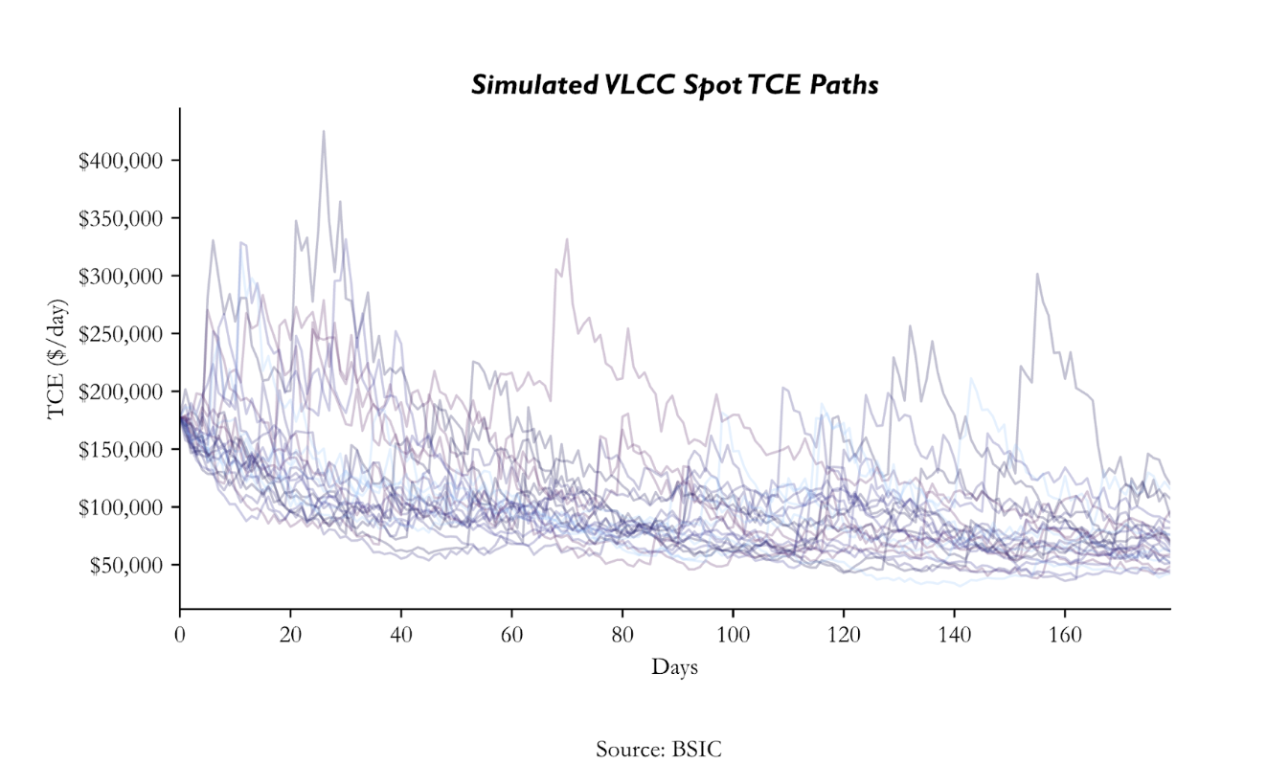The simulation shows VLCC spot TCE rates starting around ~$170k/day with high short-term dispersion, including upside spikes above $300k–$400k/day in early periods. Over the 180-day horizon, most paths mean-revert toward a ~$60k–$100k/day range, with volatility and dispersion declining over time. The distribution is right-skewed, featuring frequent normalization but occasional extreme upside shocks.

At 20 days, the mean realised forward average TCE is $92,232/day, with a median of $88,999/day and an interquartile range of $76,655–$104,714/day. At 40 days, the mean compresses modestly (low-$80k range), and by 100 days, the mean has declined to $79,658/day, with a median of $75,560/day and a 25th percentile of $61,831/day. The convergence toward ~$75k–$80k/day is gradual and consistent with the Brent curve structure discussed earlier: Freight is behaving analogously, elevated but structurally mean-reverting. Even at 100 days, the lower quartile remains materially above breakeven whilst the median declines by only 15% from 20 to 100 days ($89k to ~$75.6k). That modest compression reinforces this report’s core argument: duration, not peak magnitude, is the key variable.

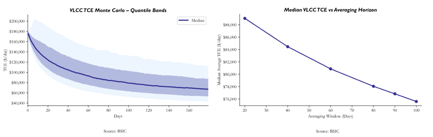The probability of sustaining an average above $200,000/day is effectively zero across most horizons. This reflects physical fleet constraints: with roughly 900 VLCCs globally (Clarksons Fleet Register), the market cannot maintain extreme scarcity pricing for extended windows absent embargo-scale capacity removal. The simulation’s cap and spike decay are consistent with historical Baltic data where crisis prints overshoot but do not define quarter-scale averages. Conversely, the probability of a realised average below $60,000/day increases from 4.34% (20 days) to 21.94% (100 days). This represents an increasing normalisation risk but $60k remains above the $37.7k breakeven, implying that even in the lower tail, vessels remain cash-generative. Moreover, the distribution skews right early and tightens left over time. This reflects empirical freight behaviour: convex in the short term and mean-reverting in the medium term.

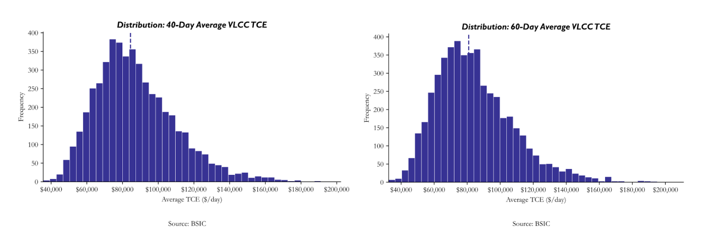Focusing on the 40–60 day horizon is appropriate given the May 29 earnings window, as this period captures the realised rate environment most relevant to near-term reported results. Across this window, the simulated mean TCE clusters around $85k–$95k/day (20-day mean: $92,232/day). Against an estimated breakeven of ~$37,700/day, this implies surplus cash generation of roughly $50k–55k per vessel per day, or approximately $18–20 million annualised per VLCC. Relative to broker-assessed asset values of $110–125 million (Clarksons/Braemar), that equates to implied unlevered cash yields of roughly 15–18%, even under moderate rate normalisation, highlighting strong near-term free cash flow visibility into earnings.

Extending to the 100-day horizon, the simulated mean moderates to $79,658/day, implying surplus of roughly $42,000/day per vessel, or approximately $15.1 million annualised. Even at this lower forward level, implied cash yields remain in the 12–14% range on prevailing asset values, indicating that free cash flow remains structurally robust well beyond the immediate earnings window. The data therefore suggest that while short-term volatility compresses over time, the longer-term distribution still supports materially positive equity cash generation above breakeven, reinforcing the convex earnings profile of tanker equities.

Applying the simulated distribution to FRO demonstrates how elevated freight translates directly into equity cash flow. With 41 VLCCs and high spot exposure, the 100-day mean TCE of ~$79,658/day implies surplus of roughly $42,000/day per vessel over an estimated $37,700/day breakeven, equating to approximately $1.7 million per day at the fleet level. Over a 90-day quarter, this translates into roughly $150–155 million of incremental VLCC free cash flow, before contributions from Suezmax and LR2 segments. Under the shorter 20-day mean (~$92k/day), surplus generation is even higher, reinforcing near-term earnings sensitivity into reporting periods. Given FRO’s near-full payout structure and scrubber penetration advantage (~$9,000/day per vessel at current spreads), realised TCE averages convert efficiently into distributable cash. The broader distribution suggests a market normalising from crisis peaks into a high-cycle plateau rather than collapsing toward breakeven: the right tail of extreme spikes is episodic, but the central tendency remains materially above solvency thresholds, while the left tail, though widening over time, still supports positive free cash flow.

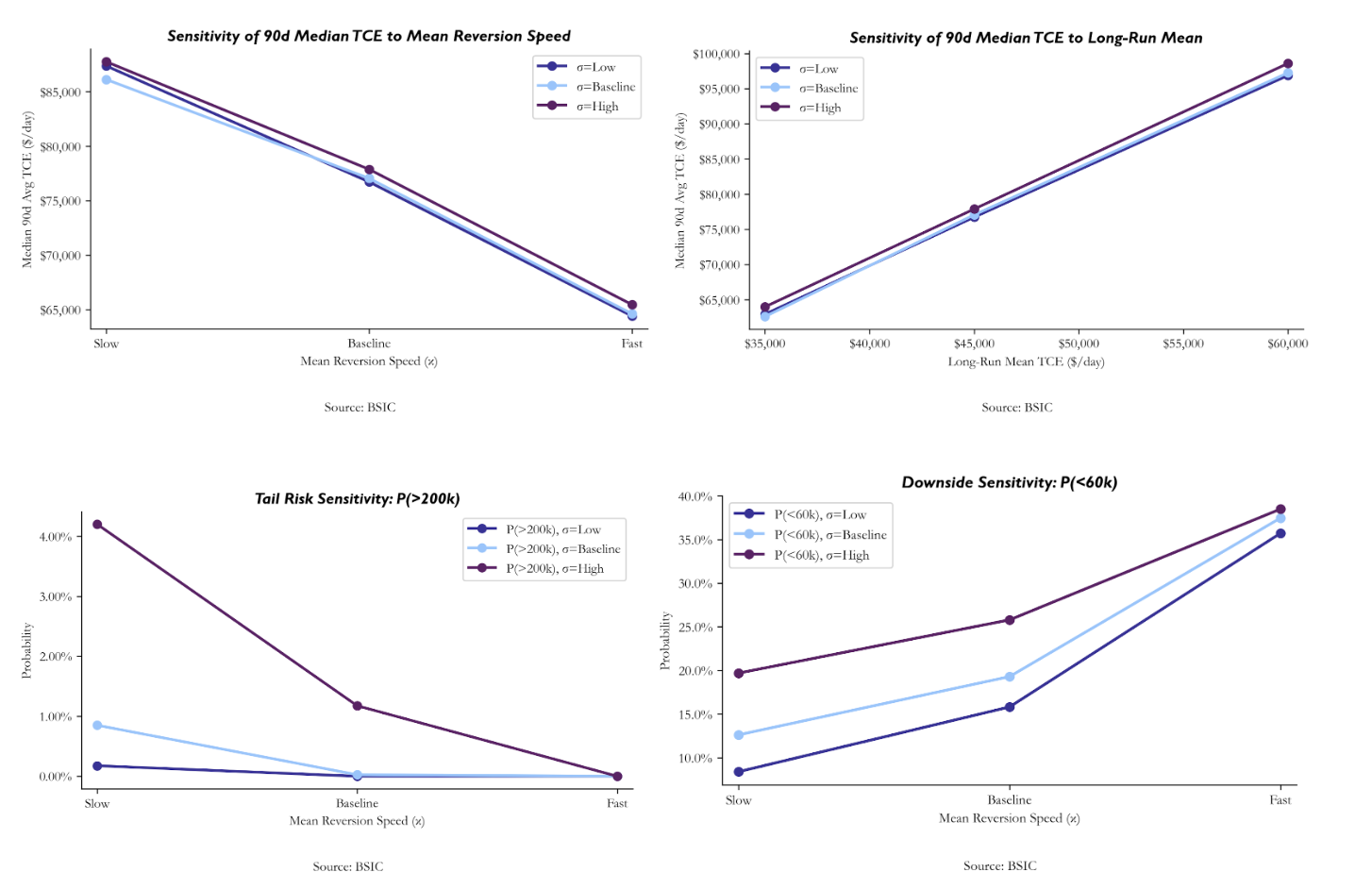Sensitivity analysis demonstrates how robust our base case is to structural changes in the underlying earnings process. In the baseline configuration (μ = $45,000, κ = ln(2)/80, σ = 0.04), the model remains as previously discussed. Varying k changed the duration of elevated earnings: slow mean reversion (120-day half-life) sustains higher TCE rates and a greater probability of right-tail probabilities. Fast mean reversion (40 day half-life) compresses forward medians to the mid-$60k region and increases the probability of sub-$60k normalisation. Adjusting long run mean of TCE shifts the earning plateau almost linearly. The graphs suggest that forward earnings are largely tethered to long-run mean reversion and half-life. Changes in volatility, (low=0.03, baseline=0.04 and high=0.06) widen dispersion in the probability of tail risk sensitivity but don’t greatly affect the median path. We can conclude from this analysis that even under faster mean reversion and higher volatility and faster mean reversion speeds, spot rates remain above break even.

Trade Expression

Accounting for our analysis of the crude oil and freight spot rate markets, we suggest FRO offers a convex risk exposure, especially given the Iran-U.S. conflict, combining maximum operational torque to the shock, with institutional liquidity and structural asset quality. The company owns one of the world’s largest VLCC fleets (41 VLCCs within an 80-vessel modernized fleet) and hence has a substantial earnings sensitivity to Middle East linked disruption, precisely where ton-mile inflation and insurance constraints are binding. The recent fleet renewal cycle, monetizing older tonnage at peak secondhand prices and rotating into scrubber-fitted ECO newbuilds, improves fuel efficiency, CII competitiveness, and asset longevity, positioning the company to command premium fixtures in a constrained environment. 

FRO operates a near-full payout model, so elevated TCE rates translate quickly into cash dividends rather than balance sheet stagnation; in a $200k/day VLCC regime, equity holders see direct yield convexity. At present the stock is not priced for sustained crisis rates, consensus anchors spot prices closer to normalized $70–80k/day, creating a valuation gap if elevated rates persist for longer than expected. At the current price of $34.56 (Mar 7), a weighting of analyst prices yields a mean target price of $37.72, an approximately 9% implied upside. Using the two bullish targets, Evercore ISI’s $46 and Fearnley’s $44 implies an $85k-$105 a day spot/TCE environment rather than a snapback implied by conservative valuations at by Clarkson’s Securities AS at $28.23 or Pareto Securities at $33.16. 

To reverse engineer the implicit VLCC spot rates we start from FRO’s share value today on March 7 and its share count, implying a market cap of about $7.7bn. With break even rates for a 5 year VLCC set at $36, 200/day, every +$10k above breakeven adds $3.65m/year per ship. With 43 VLCC set at TCE this equates to roughly $150-$160 million of incremental annual fleet cash flow. Since the equity market values tanker companies on a multiple of sustainable earnings (typically 5-6x through-cycle cash flow) that $150m supports $750-$950m of incremental equity. Thus, to move to $44 a roughly +27% in equity value, it implies an additional 2.1b in market cap. The market must thus be underwriting 2.5-3 10k/day steps above mid-cycle, implying a sustainable VLCC environment of roughly 85k-105k/day. 

In contemporary markets, Frontline plc’s equity exhibits a payoff structure that closely resembles what fixed-income practitioners term a convex bond, a return profile in which realized cash flows accelerate based on favourable moves in the underlying asset with limited retraction on adverse ones. Analogously, FRO’s realized earnings and dividend distributions can be conceptualized as a state-contingent coupon which exhibits asymmetric sensitivity to tanker freight rates. Recent industry reports document that Frontline secured seven one-year VLCC charters at approximately $76,900 per day, a level described as unprecedented in decades and indicative of a tanker market in structural imbalance between supply and demand in early 2026 in the forward freight rate market.  

Empirically, this convex payoff is revealed when comparing FRO’s observed dividend outcomes to its share price. Using recent financial disclosures, FY2025 dividend per share of $0.93 on a share price of ~$37.95 yields a trailing dividend yield of ~2.45%, a modest figure that understates underlying economics because it incorporates freight outcomes averaged across a volatile year. By contrast, the most recently declared quarterly dividend of $1.03 per share, if sustained for four consecutive quarters, annualizes to ~$4.12/share or ~10.9% yield at the same share price – an effective “coupon” more than quadruple the trailing yield – reflecting the outsized contribution of elevated freight earnings to current cash flows. In extreme stress scenarios where VLCC spot environments drive quarterly dividends into the $1.50–$2.00 range, annualized distributions of $6.00–$8.00 would imply yields in the ~15.8% to ~21.1% range at unchanged equity valuations. This illustrates an optional-like upside tied to freight persistence: small extensions in the duration of elevated freight materially amplify equity cash returns without proportionally increasing downside if freight mean-reverts.

One key risk, however, arises when NAV is the primary valuation framework for tanker equities. It represents the theoretical break-up value of the company: the aggregate market value of all vessels, less total net debt, divided by shares outstanding. In a rising rate and rising vessel value environment, NAV expands rapidly and share prices typically re-rate toward or above NAV. Vessel values are sourced from independent broker assessments (Clarksons, Braemar, Arrow). We apply the following vessel value assumptions for FRO’s fleet:

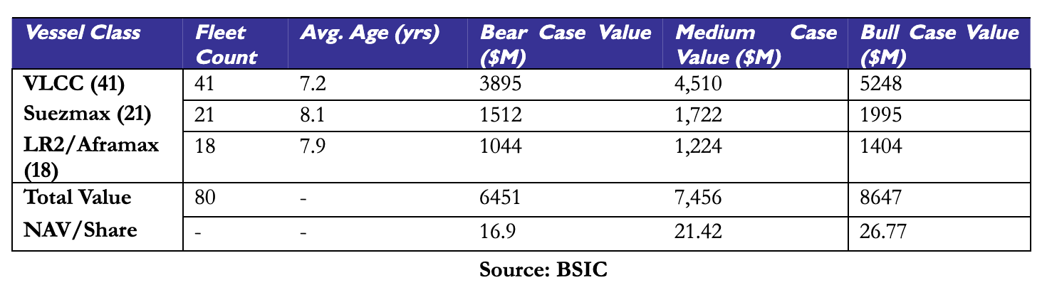
NAV derivation (using base case fleet values, FY2025 balance sheet):

Gross Asset Value (x) – Total Debt ($3,068M) + Cash & ST Inv ($253M) + Other Net Assets ($128M).

This demonstrates a price floor for FRO stock accounting for the changes in VLCC tanker prices without considering changes in the remainder of the portfolio value. In a bull case all shipping values across models would likely appreciate and total debt, cash and other net assets would likely be affected, likely leading to a substantially higher floor. The example, despite its simplicity, is illustrative of the fact that although FRO offers non-linear payoff in the event of medium term elevated freight spot prices, its downside remains capped, especially given an environment where spot price premiums bleed out of the market. 

Options Overlay

In the current market, the objective is to capture the current risk premium on oil that we estimate is priced into the 99th percentile of implied volatility (IV) and to hedge the specific “gap-up” risk that we believe to be asymmetric. In short, we are short volatility, and our view is that the market overprices the volatility of commodity price moves, except in the rare case of an upside black swan.

Instead of a traditional Iron Condor or a naked Strangle, we recommend a 30-delta hybrid strategy. This structure involves selling a 30-delta OTM Put (naked), selling a 30-delta OTM Call, and buying a 10-delta OTM Call as a protective wing.

Our intuition relies on the nature of tail risk. In the current market, in fact, an upside move in oil price is the real risk to consider. If a major chokepoint like the Strait of Hormuz is blocked, oil prices will violently jump. A naked short call in that scenario could lead to liquidation before having the chance to delta-hedge. The 10-delta protective call acts as a hard ceiling, stopping potential losses while our long FRO (Frontline) equity position captures the resulting increase in freight rates.

Conversely, the downside behaves differently. While oil can drop as the war premium may fade over time, it rarely gaps violently in a single session. This provides time to manage a naked short put by either rolling the position or selling futures to delta-hedge. By skipping the protective put, we avoid overpaying for a very expensive premium in a high IV environment. This may allow us to profit more aggressively from the eventual volatility crush.

Conclusion

The current conflict between Iran and the U.S. has already caused a short-term supply disruption to the oil and tanker markets. However, the real question is how long this disruption will last. Freight rates may stay high due to war-risk insurance costs, re-routing of vessels, longer transit times and uncertainty. That said rates could easily collapse in the event of a quick de-escalation of the crisis or if the higher oil prices drive demand destruction, although unlikely.

It is our view that spot freight rates look to remain elevated, especially for the coming month. FRO has large exposure to crude tanker shipping, and its business model is aligned to capture a large portion of the value from the aforementioned geopolitical events, translating into significant free cash flow additions. In the current risk environment, we believe this FRO equity play is best combined with an options overlay to protect against either a sharp up move in crude in the near term, or a reversal of the war premium that is currently built into spot rates.

References

[1]  Alizadeh, Amir H., and Nomikos, Nikos K., Shipping Derivatives and Risk Management, 2009

[2] Baltic Exchange, VLCC Health of Earnings Index (2Q24 Methodology Report), 2024

[3] Baltic Exchange, Tanker Route Assessments (TD3C Historical Series), Various Years

[4] Braemar (Arrow), Secondhand Tanker Market Assessments, 2026

[5] Clarksons Research, Fleet Register and VLCC Orderbook Data, 2026

[6] Clarksons Research, Tanker Earnings Time Series, Various Years

[7] Clarksons Research, Secondhand Vessel Valuation Reports, 2026

[8] House of Commons Library, Israel and the U.S. Strike Hundreds of Targets: Nuclear Sites and Missile Launchers Hit in the First Wave, 2026

[9] Lloyd’s List Intelligence, Global VLCC Earnings Reports, 2026

[10] Lloyd’s of London Joint War Committee, Listed Areas – Persian Gulf, Strait of Hormuz, Gulf of Oman, 2026

[11] Fars News Agency, IRGC Launches “Operation True Promise 4”: Hundreds of Missiles Target U.S. Bases, 2026

[12] Caspian News, Iran State TV Confirms Khamenei “Martyred”; 40 Days of Mourning Declared, 2026

[13] Polymarket, Event Contracts: US–Iran Ceasefire, Strait of Hormuz Closure, US Forces Enter Iran, 2026