Attention Factors

Download PDF

Introduction

In this article we present a conditional latent factor approach to decompose US equities returns into systematic latent components and idiosyncratic residuals. The aim of the article is to expand on previous research by the Bocconi Student Investment Club by presenting an alternative approach to the traditional PCA decomposition.

We implement the Attention Factor Model of Epstein, Wang, Choi and Pelger (ICAIF 2025) on a universe of 200 US equities from 2010 to 2017. The model replaces the fixed eigenvectors of PCA with a learned factor structure: a cross-attention mechanism groups stocks into K latent factors based on time-varying firm characteristics, extracts idiosyncratic residuals, and then a long convolution (LongConv) sequence model is implemented to extract signals from the residuals’ time-series to construct a factor-neutral statistical arbitrage portfolio.

We first motivate the shift from static to conditional factor models. We then present the full mathematics of the attention decomposition, the LongConv alpha engine, and the portfolio construction pipeline, illustrating each step with numeric examples drawn from the equities implementation. Finally, we discuss the out-of-sample results and interpret what the model has learned.

Differences and advantages from the PCA approach

The classical statistical arbitrage framework decomposes the N-dimensional return vector R(t) into a systematic component and an idiosyncratic residual via PCA. Concretely, one estimates the covariance matrix of returns over a trailing window, extracts its top K eigenvectors to form a loading matrix B of shape (N, K), and defines the residual as ε(t) = R(t) − B(BᵀB)⁻¹BᵀR(t). The residuals are then modelled as mean-reverting processes to generate trading signals.

This approach has three structural limitations. First, PCA eigenvectors are unconditional: they are estimated from the data matrix alone and do not vary with observable characteristics such as momentum, volatility, or size. If the factor loadings shift when a stock transitions from low-volatility to high-volatility, PCA uses the same static eigenvector, forcing the operator to frequent recalibration. Second, the eigenvectors are constrained to be mutually orthogonal, which is a mathematical convenience rather than an economic prior. There is no reason to believe that the true factor structure of equity returns involves perpendicular loading vectors. Third, PCA is an unsupervised decomposition: it maximises explained variance without regard to whether the resulting residuals are tradeable. This final point is crucial for this research, a simple strategy applied to mean reverting residuals with PCA can solicit a tremendous turnover of long and short positions, which is clearly inapplicable due to transaction costs.  

The Attention Factor Model addresses all three. Factor loadings are conditional on M time-varying firm characteristics at each time step, so a stock’s factor exposure changes as its characteristics change. The learned weight vectors have no orthogonality constraint, allowing correlated or overlapping factors. And the entire model is trained end-to-end with a loss function that jointly maximises portfolio Sharpe ratio after transaction costs and explained variance, so the factor structure is shaped by what is both economically meaningful and tradeable.

How the model learns: a brief primer on the Machine Learning process

Before diving into the model’s architecture, it helps to understand the general machine learning mechanics that the model subtends. Every learnable component in this model (the embedding matrix W_K, the factor queries Q, the convolution kernels K, the portfolio head) is just a collection of vectors or matrices which undergoes random initialisation and gets iteratively adjusted according to a specified rule. Three concepts are essential: parameters, the loss function, and gradient descent.

A parameter is any value the model is allowed to change during training. Our model has roughly 2,500 learnable parameters grouped into matrices and vectors. At initialisation, every one of these numbers is drawn from a random distribution, typically a scaled uniform or normal distribution (order 0.01 to 0.5). The model at this point is meaningless: the factors group stocks randomly, the attention weights are uniform, and the forecasts are noise.

Consider one row of W_K (the weights that determine how “ret_1d” contributes to each of the 32 embedding dimensions). At initialisation it might be:

After 80 epochs of training, the same row might look like:

Dimension 0 grew from +0.12 to +0.48 because the optimiser found that a strong ret_1d contribution to dimension 0 helps separate momentum stocks from mean-reverting stocks. Dimension 2 shrank from +0.31 to +0.03 because ret_1d was not useful in that dimension. Every number in every matrix undergoes this kind of adjustment.

The loss function produces an output value that measures the deviations of the model’s performance from the target predictions. The model’s job is to minimise this output. 

In our case:

The negative sign flips maximisation into minimisation: a higher Sharpe ratio and higher explained variance both make the loss more negative, which is what the optimiser seeks. The coefficient 5.0 controls the relative importance. At initialisation, with random parameters, the Sharpe ratio is near zero and the explained variance is near zero, so the loss is approximately −(0 + 5.0 × 0) = 0. After training, a well-fitted model might have Sharpe ≈ 3.0 and explained variance ≈ 0.18, giving loss ≈ −(3.0 + 5.0 × 0.18) = −3.9. The optimiser drove the loss from 0 to −3.9 by adjusting every parameter.

Gradient descent is the process  of modern machine learning that can compute, for every single parameter, the gradient: how much would the loss change if we nudged this parameter by a tiny amount? This is computed via automatic differentiation (backpropagation), which applies the chain rule through every operation in the forward pass.

Once we have the gradient for every parameter, the update rule is simple. For each parameter θ:

If the gradient is positive (increasing the parameter would increase the loss, i.e. make things worse), we decrease the parameter. If the gradient is negative (increasing it would decrease the loss, i.e. improve things), we increase it. The learning rate (lr = 10⁻³ in our model) controls the step size. We use AdamW, a variant that also tracks the history of past gradients to set an adaptive step size per parameter and applies weight decay (0.05) to gently shrink parameters toward zero unless the gradient actively pushes them away.

Suppose W_K[ret_1d, dim_0] = +0.12 at the start of an epoch. One “epoch” is a full pass through the training data. The forward pass runs: characteristics are embedded, factors are computed, residuals are extracted, LongConv forecasts positions, the portfolio earns returns, and the loss is computed. Backpropagation traces the chain: “if W_K[ret_1d, dim_0] were slightly larger, the embedding for high-momentum stocks would shift, changing their attention scores, affecting the factor returns, modifying the residuals, altering the LongConv input, which would change signals, ultimately affecting the Sharpe ratio.” Suppose the result is gradient = −0.36, meaning increasing this parameter would decrease the loss (improve performance). The update: θ_new = 0.12 − 0.001 × (−0.36) = 0.12 + 0.00036 = 0.12036. A tiny nudge upward. Over 80 epochs with hundreds of such steps, the parameter migrates from +0.12 to +0.48.

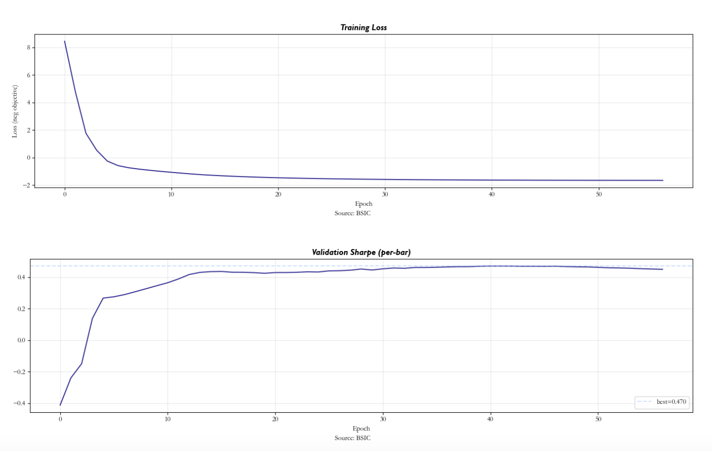
Our model trains for up to 80 epochs with early stopping: if the validation Sharpe ratio does not improve for 15 consecutive epochs, training halts. We also use a warmup phase: for the first 10 epochs, only the explained-variance term of the loss is active (Sharpe weight = 0). This gives the factor model time to learn a reasonable decomposition before the portfolio optimiser starts pushing parameters. Without warmup, the Sharpe gradient can overwhelm the factor-learning gradient in early epochs, leading to a degenerate solution where no factors are learned and LongConv tries to predict raw returns.

Every forward pass produces a loss. Every loss produces gradients for all ≈2,500 parameters simultaneously. Every parameter takes one small step in the direction that reduces the loss. After thousands of such steps, the random initial matrices have been sculpted into a factor model that captures real cross-sectional structure and a LongConv that predicts residual dynamics. The next sections walk through each component of this pipeline, showing the matrices and vectors at each step.

Model implementation

Firm characteristics and rank normalisation

At each trading day t, we observe M = 18 characteristics for each of N = 200 stocks. These span short-term microstructure signals (1-day return, overnight gap, intraday high-low range, volume ratio vs 63-day moving average), medium-horizon features (5-day and 21-day returns, 21-day realised volatility, price deviation from 21-day MA, maximum return over 21 days, Amihud illiquidity), long-horizon features (63-day and 126-day returns, Jegadeesh-Titman 12-1 month momentum, 63-day volatility, deviations from 63-day and 252-day MAs), and cross-sectional features (log price level, dollar volume size rank).

The original Epstein et al. paper uses a considerably richer feature set, including fundamental characteristics such as profitability ratios, earnings yield, price-to-earnings, book-to-market, asset growth, and investment intensity, several dozen features in total drawn from the comprehensive cross-section used in the asset pricing literature. In our implementation, we restrict the feature set to 18 purely technical and market-microstructure characteristics. This choice reflects the data available for our universe and time period; extending to fundamental features would be a natural next step and would likely improve the factor decomposition’s ability to capture value, quality, and profitability-driven systematic risk.

We rank-normalise each characteristic cross-sectionally at every time step. For each feature m, the N stock values are ranked and divided by N to produce values in [0, 1]. This eliminates scale differences across features: a 5% daily return and a $50 billion market cap become comparable rank-percentiles.

Consider N = 4 stocks and M = 3 characteristics at one day. The raw characteristic matrix X_raw (shape 4 × 3):

After rank-normalising each column independently (rank ÷ N), the matrix X(t) becomes:

Each row is one stock’s feature vector; each entry is now a rank-percentile in [0, 1]. The full model produces X(t) of shape (200, 18) at every trading day.

Embedding characteristics via W_K 

The key projection matrix W_K has shape (M × d) = (18 × 32). Each of the d = 32 columns defines a learned linear combination of the 18 raw characteristics. For stock n at day t:

Each dimension of the embedding is a custom blend of characteristics. For instance, dimension j might compute 0.31 · ret_1d − 0.22 · vol_21d + 0.15 · ma_dev_21d + … across all 18 features. These blends are not orthogonal (unlike PCA components), not ranked by variance, and are trained end-to-end through the loss function. The model uses d = 32 > M = 18, giving the query vectors more directions to work with than there are raw features. Some dimensions end up near-zero (unused), which is acceptable: spare capacity is cheaper than constraining the model.

In the toy case with M = 3 and d = 4, suppose W_K at initialisation is the following (3 × 4) matrix of random values:

For AAPL with rank-normalised features x = [0.75, 0.50, 0.75], the embedding is the matrix-vector product x · W_K. Dimension 0: 0.75 × (+0.31) + 0.50 × (−0.22) + 0.75 × (+0.15) = +0.23 − 0.11 + 0.11 = +0.23. Computing all four dimensions gives the embedding vector:

Computing the same product for all four stocks gives the full embedded matrix E(t) = X(t) · W_K of shape (N × d) = (4 × 4):

Each row is one stock’s position in the d-dimensional embedding space. In the full model, E(t) has shape (200, 32) and changes at every trading day as the characteristics evolve. Stocks with similar characteristics produce similar embeddings and land near each other.

Factor queries and attention scores

The query matrix Q has shape (K × d) = (5 × 32). Each row Q(k) is a “factor template” that defines what factor k looks for in embedding space. For each factor k and stock n, the attention score is the scaled dot product:

The division by √d = √32 ≈ 5.66 prevents the dot products from growing large with d, which would cause the subsequent softmax to saturate. The scores form a matrix of shape (K × N) = (5 × 200).

Example. In the toy case with K = 2 factors and d = 4, the Q matrix (2 × 4) at random initialisation:

score(0, AAPL) = Q(0) · AAPL_emb / √4 = (0.22 × 0.23 + (−0.35) × (−0.12) + 0.18 × 0.56 + 0.41 × 0.23) / 2 = 0.291 / 2 = 0.146. At initialisation, all scores are small and similar because W_K and Q contain random values.

Softmax attention weights

For each factor k, the softmax across the N stocks converts scores into a probability distribution:

This gives ω(k) as a vector of N non-negative weights summing to 1. At initialisation the weights are nearly uniform (each ≈ 1/200 = 0.005 for 200 stocks) because the random scores are small. After training, a trained factor might concentrate most weight on 10–20 stocks that genuinely co-move, with the rest receiving near-zero weight. The matrix ω of shape (K × N) = (5 × 200) is the attention weight matrix: it tells us which stocks belong to which factor, with soft (not hard) assignments.

Factor returns

Crucially, the attention weights use characteristics from day t − 1 applied to returns at day t, ensuring no look-ahead bias. The return of factor k at day t is the attention-weighted average of stock returns:

If the daily log-returns are R = [−0.02, +0.01, −0.03, +0.04] and factor 0’s attention weights (from yesterday’s characteristics) are ω(0) = [0.254, 0.240, 0.260, 0.246], then f(0) = 0.254 × (−0.02) + 0.240 × 0.01 + 0.260 × (−0.03) + 0.246 × 0.04 = +0.0003. At initialisation both factors return nearly the same value because the uniform weights average everything out. After training, factors capture different systematic drivers and produce distinct return series.

Factor loadings via ridge regression

Given the K factor returns, we need each stock’s loading (beta) on each factor. Rather than running N separate regressions, the closed-form ridge solution gives all betas simultaneously:

The ridge term λ_ridge = 10⁻³ prevents the Gram matrix from being singular. The resulting β(n, k) tells us how much stock n moves per unit move in factor k. This is computed at each time step (since ω changes daily), making the loadings time-varying and conditional on characteristics.

Extracting residuals

The fitted return and residual for stock n at day t are:

ε(t, n) is the idiosyncratic residual: the part of stock n’s return that the K factors cannot explain. This is what the LongConv module will interpret. Importantly, when feeding residuals into LongConv, we shift them by one day (ε at position i uses data through day i − 1 only) to maintain strict causality: the trading signal at day t never uses the return at day t.

Long convolution on residuals

Each stock’s scalar residual is first projected to d = 32 channels via a linear layer: h(t, n) = residual_proj(ε(t, n)), producing a (1,) → (32,) expansion. This is simply 32 learned multipliers applied to the same scalar. If ε = −0.05 and the weights are [+2.1, −0.8, +0.3, …], then channel 0 sees −0.105, channel 1 sees +0.040, and so on. Same information at different scales and signs, giving each channel a different starting point.

For each channel h and each stock independently, LongConv computes a weighted sum over the past L = 30 days of that channel’s history:

where K_h is the learned kernel (30 weights for channel h) and D_h is a separate skip-connection weight. The convolution is implemented via FFT for efficiency: Y = IFFT(FFT(input) × FFT(kernel)), which computes the identical result in O(T log T) instead of O(T × L).

The Kernel initialisation is the only non-random initialisation in the model. Each channel gets an exponential decay envelope with a different decay rate: decay_rate(h) = 16^(h/32). Channel 0 (rate = 1.0) starts with non-zero weights at all 30 lags and can “see” the full history. Channel 31 (rate ≈ 14.6) has its envelope effectively zero after lag 2–3, so it starts as an ultra-short-term filter. The random values inside each channel are truly random (drawn from a standard normal), but the envelope that scales them is deterministic and different per channel. This gives the optimiser a multi-resolution starting point rather than requiring it to discover timescale separation from scratch.

After every optimiser step, each kernel weight undergoes soft-thresholding: K_h(j) ← sign(K_h(j)) · max(|K_h(j)| − 0.001, 0). Every training step, each weight loses 0.001 of magnitude. Only weights that the gradient keeps pushing away from zero (because they improve the loss) survive. After training, most of the 32 × 30 = 960 kernel entries are exactly zero. The surviving non-zero entries are the lags that carry genuine signal.

Suppose after training, channel 0’s kernel has converged to mostly zeros with a few survivors: lag 1 = −0.42, lag 2 = −0.18, lag 15 = +0.11, lag 16 = +0.08, all others zero. At day t, if channel 0’s input history has h(t−1) = +0.30, h(t−2) = +0.15, h(t−15) = +0.20, h(t−16) = +0.25, then output = (−0.42)(0.30) + (−0.18)(0.15) + (0.11)(0.20) + (0.08)(0.25) = −0.108. The negative weights at recent lags encode short-term reversal; the positive weights at lag 15–16 encode a slower pattern roughly 3 weeks back. The net negative output signals “go short on this stock.”

Inspecting the surviving (non-zero) kernel weights across the 32 channels reveals a consistent pattern. Channels initialised with slow decay (low h) retain weights at lags 1–5 with negative sign (short-term reversal) and sometimes positive weights at lags 15–25 (a slower mean-reversion pattern). Channels initialised with fast decay (high h) typically converge to a single non-zero weight at lag 1, acting as a simple AR(1) filter. The portfolio head then combines these “fast” and “slow” channels into a blended signal.

After the convolution, each stock has 32 channel outputs. A linear head (32 → 1) combines them into a single forecast: forecast(t, n) = α_0 · ch0_out + α_1 · ch1_out + … + α_31 · ch31_out. The mixing weights α are learned, so the model can upweight channels that have found useful patterns and effectively zero out channels that produce noise. 

Factor-neutral portfolio construction

The LongConv forecasts are raw portfolio weights w_raw(t). These might inadvertently bet on the factors. To ensure the portfolio captures only idiosyncratic alpha, we orthogonalise against the factor space:

The inner product βᵀ w_raw gives the portfolio’s exposure to each factor (a K-vector). Multiplying by ωᵀ projects this exposure back to asset space, and subtracting it removes the factor bet. The result w_asset has exactly zero net exposure to all K factors.

With K = 2 and N = 4, the raw weight vector from LongConv and the beta loading matrix are:

The raw portfolio’s exposure to factor 0: βᵀ(:, 0) · w_raw = 0.80 × (−0.065) + 0.10 × 0.120 + 0.60 × (−0.030) + 0.30 × 0.045 = −0.044. Similarly for factor 1: +0.085. The adjustment vector ωᵀ · [−0.044, +0.085] redistributes this exposure across stocks; subtracting it yields w_asset with exactly zero exposure to both factors.

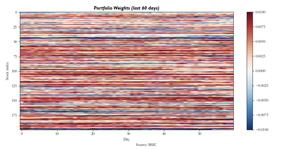
Finally, the weights are L1-normalised (w_norm = w_asset / Σ|w_asset|) to make the portfolio dollar-neutral with total absolute weight 1.

Transaction costs and net returns

The gross portfolio return at day t is the inner product of yesterday’s weights with today’s returns: gross(t) = Σ_n w_norm(t−1, n) · R(t, n). Transaction costs are proportional to turnover: TC(t) = c · Σ_n |w_norm(t, n) − w_norm(t−1, n)|, where c = 4 bp per unit of turnover. Net returns are simply net(t) = gross(t) − TC(t). These net returns are what the Sharpe term of the loss function optimises.

A key practical advantage of this architecture is its natural compatibility with real-world market microstructure. In live execution, different stocks have vastly different bid-ask spreads and order book depths: a highly liquid large-cap like AAPL might trade at a 1 bp effective spread, while a mid-cap with thinner depth of book may cost 8–15 bp per round trip. Because the factor-neutral construction already dampens turnover (factor exposure adjustments are smooth functions of slowly changing characteristics), and because the LongConv kernel squashing drives most kernel weights to zero (producing a sparse, low-frequency signal), the strategy naturally generates moderate turnover. This makes it well suited for diverse universes where trading costs vary substantially across the order book.

In our implementation, we do not have access to tick-level bid-ask spread data or intraday volume profiles for the full 2010–2017 sample, so we proxy transaction costs with a flat rate of 4 bp per unit of turnover. This is a conservative estimate for the universe of 200 liquid US equities considered: empirical studies of effective spreads for large- and mid-cap US stocks over this period typically report median half-spreads in the 2–5 bp range. A production deployment would replace this flat proxy with stock-specific cost models calibrated to realised spreads and volume participation rates, which would likely improve net performance for the most liquid names while tightening risk controls on the least liquid ones.

Training objective

We finally define the loss function that jointly optimises portfolio performance and factor quality:

where ExplainedVariance = mean over stocks of (1 − Var(ε) / Var(R)), computed as temporal variance per stock. The hyperparameter λ_var = 5.0 ensures that the factor decomposition learns to capture real systematic variance rather than collapsing to a trivial solution. Without this term, the model could set all factor weights to zero (making ε = R) and rely entirely on LongConv to predict raw returns — which is much harder than predicting residuals after removing common factors.

The Sharpe term shapes LongConv and the portfolio head toward profitable trading. The ExplainedVariance term shapes W_K and Q toward meaningful factor structure. All parameters update simultaneously via AdamW (lr = 10⁻³, weight decay = 0.05) with a warmup phase: for the first 10 epochs, only the ExplainedVariance term is active, giving the factor model time to learn a reasonable decomposition before the Sharpe term introduces trading pressure.

Once factor 0 captures, say, the co-movement among large-cap tech stocks, those stocks’ residuals shrink. Factor 1 gets no explained-variance benefit from also attending to the same group, their variance is already explained. Factor 1’s gradient instead pushes it toward the remaining unexplained variance, perhaps the co-movement among energy stocks or small-cap value names. This implicit competition for unexplained variance drives each factor to find a distinct cluster.

Results

We apply the model to a universe of N = 200 US equities selected by median dollar volume from the full CRSP-style daily dataset over 2010–2017. We use M = 18 firm characteristics, K = 5 factors, d = 32 hidden dimensions, and L = 30 day lookback for LongConv. The data is split 75/10/15 into train, validation, and test sets. Training uses a 504-day (2-year) batch window for stable Sharpe estimation, with early stopping (patience = 15 epochs) on validation Sharpe.

To validate robustness, we run a rolling walk-forward backtest: train on 504 days (2 years), test on the next 21 days (1 month), slide forward by 21 days, and retrain from scratch at each step. Every test-period return is strictly out-of-sample. The walk-forward framework tests whether the model’s learned dynamics generalise beyond the training window.

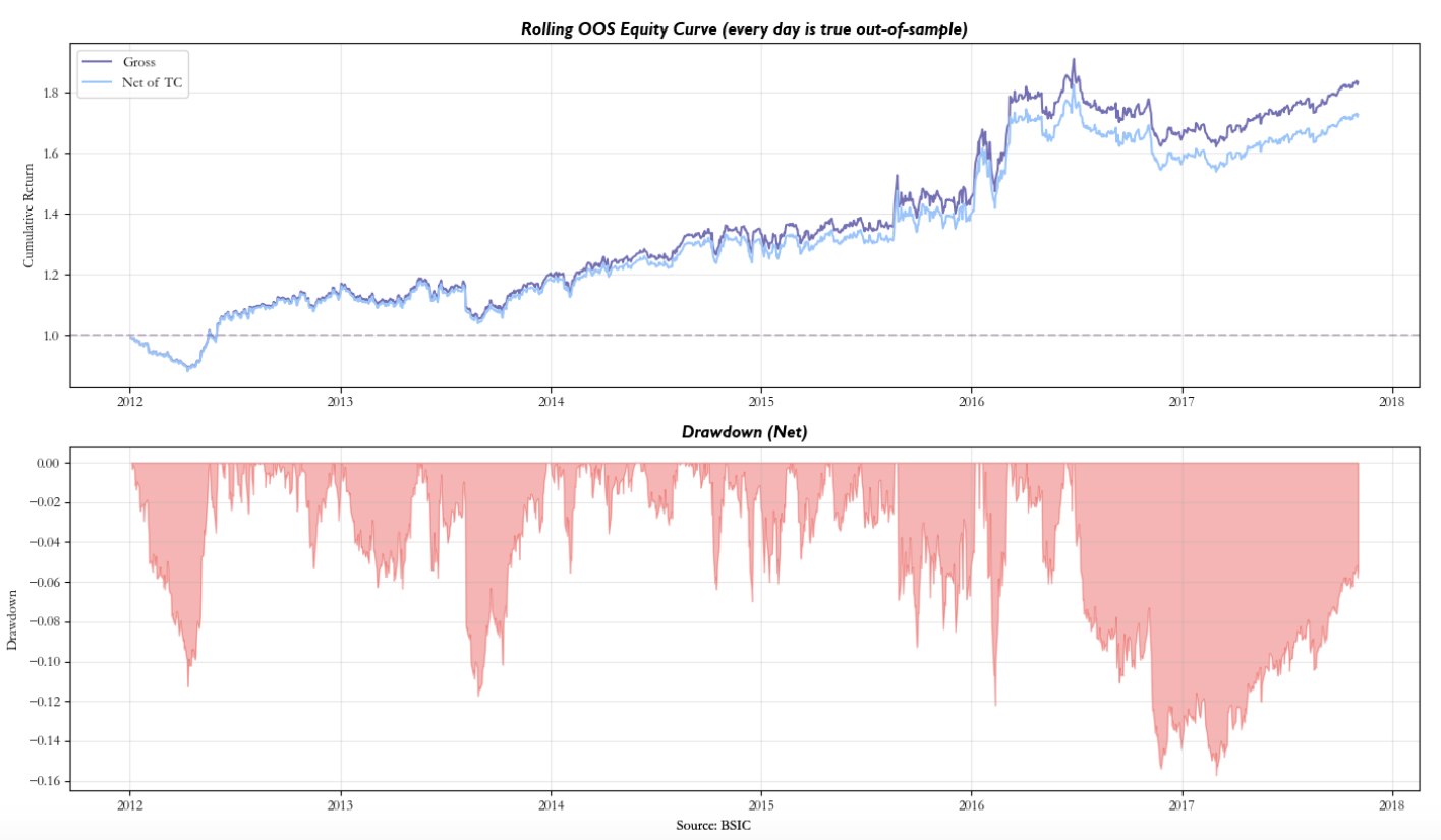
The strategy yields a Sharpe Ratio after transaction costs of 0.78, with annualised returns 10.2% and annualised volatility 13.2%. 

It appears that the pipeline was able to somewhat remove the systematic component driving the returns and that the LongConv process was able to detect through its channels some mispricing. In fact, recalling the factor investing basics, the strategy profits when individual stock residuals exhibit predictable temporal dynamics, short-term mean reversion, slow drift, or regime-dependent patterns that a linear combination of lagged residuals can exploit. 

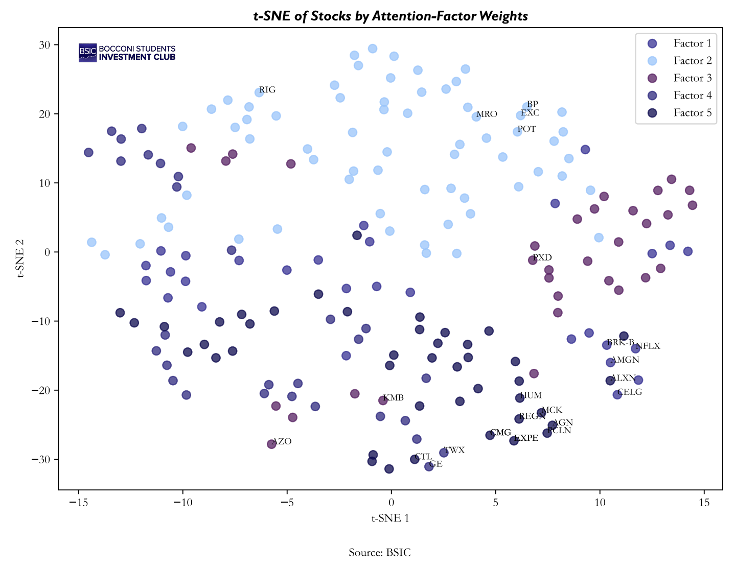
Provided that the backtest yielded some positive results it is of higher importance to understand if the model was able to capture some significant latent factors. We use graph theory and t-distributed stochastic neighbourhood embedding (t-SNE) to qualitatively control the results. 

We initially present a distance correlation network, constructed directly from raw returns. As expected the unconditional dependence across assets presents a close affiliation to sectoral classifications, capturing the well-known structure of equity returns comovements.

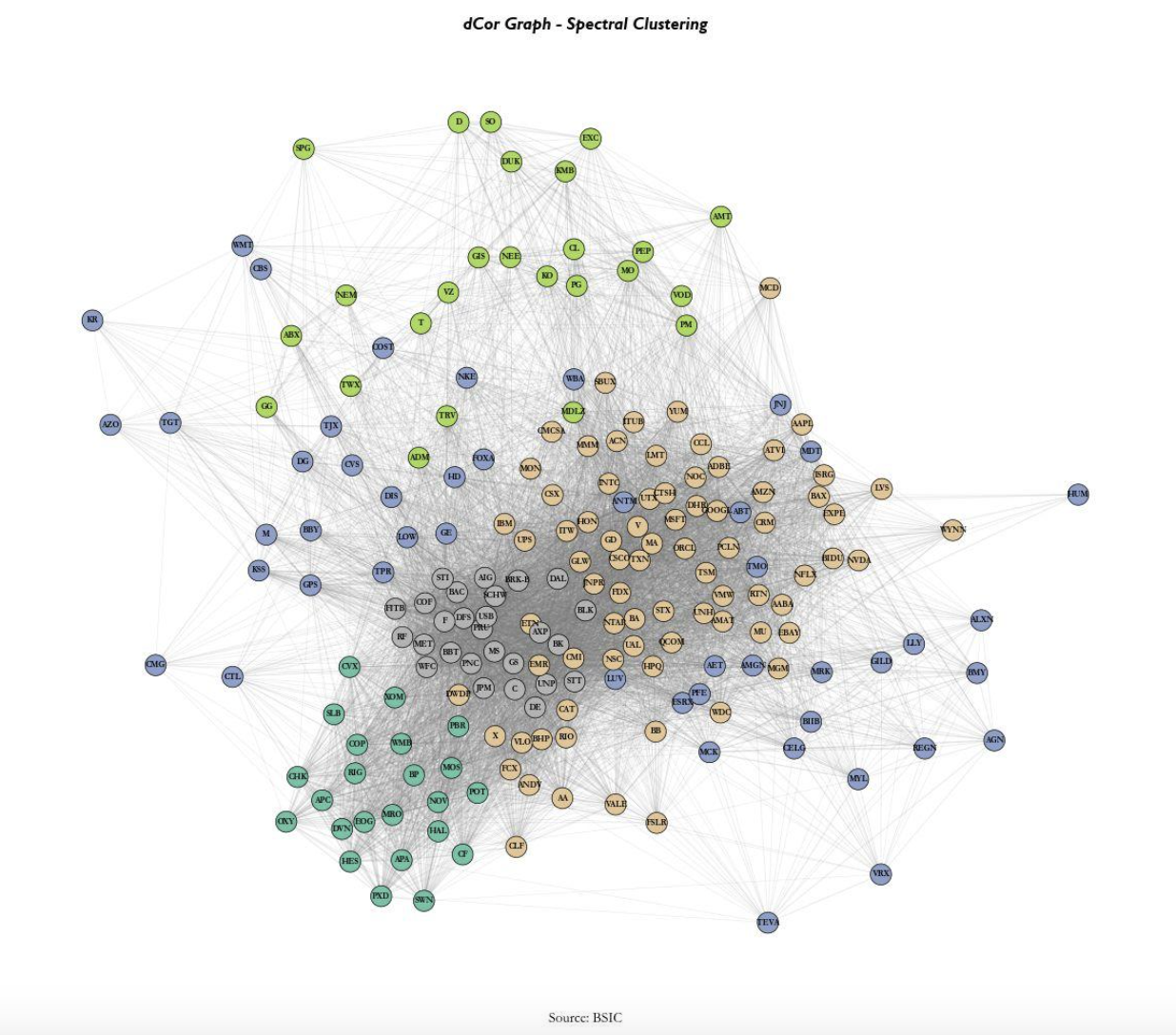
In contrast, the t-SNE derived directly from the latent factor loadings produced by the model represents the learnt similarities between after the model’s conditioning. While some sector level grouping is still visible, the embedding exhibits additional dispersion within clusters, suggesting that the model differentiates assets along dimensions which aren’t captured by simple return correlation.  If the model were not learning meaningful latent factors, the t-SNE representation would largely replicate the structure observed in the dCor graph. The observed deviations therefore provide qualitative evidence that the model captures additional cross-sectional information beyond static correlation.

Finally, stocks with similar factor loadings tend to cluster locally, indicating that the learned latent factors lead to a coherent grouping in the representation space. At the same time, these clusters are not perfectly separated and often overlap, suggesting that assets are influenced by multiple factors simultaneously rather than belonging to a single discrete group. This contrasts with the sharper sectoral segmentation observed in the distance-correlation network and is consistent with the notion of conditional latent factors that capture nonlinear dependencies.

References

1. Epstein, S., Wang, C., Choi, J. and Pelger, M., “Neural Attention Factor Models for Statistical Arbitrage”, ICAIF 2025
2. Avellaneda, M. and Lee, J.H., “Statistical Arbitrage in the US Equities Market”, Quantitative Finance, 2010