Smile (and skew) for the camera!

Introduction

Across different asset classes, volatility surfaces all tell different stories: in this article we let the data tell them unfiltered, building each surface directly on market quotes through interpolation rather than through the lens of a parametric model. Implied volatility surfaces are among the most informative objects in option markets, capturing the market’s comprehensive view of risk across strikes and maturities at a given moment in time in a single three-dimensional structure. In order to understand the factors driving the differences examined further, it is worth starting from the theoretical foundation contextualising a volatility surface in the first place.

Options pricing has its historical base in the Black Scholes model. Introduced by Black and Scholes in 1973 and later extended by Merton, the model, assuming that the underlying asset follows a geometric Brownian motion with constant volatility over time and for every strike and expiration date, gives a closed form formula for the price of a European option. More specifically, for a European call option: $C_{BS}(S_0, K, T, r, q, \sigma) = S_0 e^{-qT} N(d_1) - K e^{-rT} N(d_2)$ , where $d_1 = \frac{\ln(S_0/K) + \left(r - q + \frac{\sigma^2}{2}\right)T}{\sigma\sqrt{T}}, \qquad d_2 = d_1 - \sigma\sqrt{T}$ and $S_0$ is the current asset price, $K$ the strike, $r$ the risk-free rate, $T$ the time to maturity, $\sigma$ the volatility, and $N(\cdot)$ the standard normal CDF. Despite providing an elegant solution for options pricing, it is widely acknowledged that B-S assumptions fail to hold in the real world. However, its limitations can be the starting point to understand volatility surfaces. To start with, volatility is treated as a scalar parameter in the model: therefore, when inverting the BS formula on market prices $C_{mkt}(K,T)$ , we obtain the implied volatility, not as scalar, but as a function of strike and maturity, $C_{BS}(S_0,K,T,r,q,\sigma_{IV}) = C_{mkt}(K,T)$ , the volatility that satisfies this equation. Contrary to what is assumed with the B-S model, implied volatility varies across the pairs (K,T) available in the market, in a systematic and structured way.

The volatility surface collects these values, visualized as a three-dimensional surface with:

X-axis: strike K, or log-moneyness $m = \ln\left(\frac{K}{S_0}\right)$ , the convention adopted here which centers the surface on ATM;
Y-axis: time to maturity T (in years, from short to long-term), i.e. $T = \frac{\text{expiration date} - \text{observation date}}{365}$ ;
Z-axis: implied volatility, $\sigma_{IV}$ , simply the ‘height of the surface in that point’;

More specifically the volatility surface follows this map: $\sigma_{IV} : (K, T) \mapsto \mathbb{R}_{>0}$ . Every point on the surface addresses the question: “At which volatility is the market pricing an option with this price and this maturity?”

The surface can be read along two dimensions. Fixing a maturity T and slicing the surface vertically yields the volatility smile for that expiry showing how implied volatility varies across strikes at a given point in time. Fixing a strike K and slicing in the other direction yields the term structure of volatility showing how implied volatility evolves across maturities for a given moneyness level.

As mentioned above, implied volatility is not flat across strikes. However, the variation is structured and has a specific economic meaning: the cross-sectional shape of the surface directly reflects the risk-neutral distribution of the underlying, that is, the probabilities that the market implicitly assigns to different future price levels when pricing options today. This essential link is formalized by the Breeden-Litzenberger theorem, according to which the risk-neutral density is proportional to the second derivative of the call price with respect to strike,

$p_T(K) = e^{rT} \frac{\partial^2 C(K,T)}{\partial K^2}$ , showing that option prices (and volatility surfaces) embed the market-implied distribution of future prices.

A volatility surface can be interpreted through three key features: the volatility smile, the skew, and the term structure, all varying across asset classes depending on the underlying risk profile, market structure and the nature of demand for hedging. The volatility smile describes how implied volatility varies across strikes for a fixed maturity, typically displaying higher values for deep in- and out-of-the-money options. The skew refers to the asymmetry of this pattern, particularly evident in equity markets where implied volatility is higher for low strikes, reflecting greater concern for downside risk. The term structure instead captures how implied volatility changes across maturities for a given level of moneyness, providing information about how uncertainty evolves over time. Therefore, from the perspective of the B-L theorem, a smile signals fat tails (i.e. higher kurtosis) on both sides of the distribution: in other words, the market prices options as if large upward and downward movements were more likely than in a lognormal context. Furthermore, a skew with a surface sloping downward toward OTM puts, signals asymmetric tail risk pricing: investors structurally long equity bid up OTM puts as crash protection, inflating their implied volatility relative to OTM calls at the same distance from ATM. These shapes matter because any strategy involving options at different strikes, spreads, risk reversals or exotic payoffs, is directly exposed to them. Pricing with a flat surface produces systematic errors in delta, in hedge ratios, and in the valuation of non-linear payoffs.

In trying to overcome the limitations posed by B-S and model volatility more realistically, research has produced numerous useful models. To cite some of them, the first two specify richer dynamics for the underlying, calibrating the parameters of a stochastic process to reproduce the observed surface, while the last ones are direct parametric representations of the surface itself:

Stochastic Volatility – Heston, 1993: introduces stochastic variance with mean reversion and correlation between spot and volatility; provides a semi-closed-form solution and is widely used for equity and FX markets;
SABR (Stochastic Alpha Beta Rho) – Hagan et al., 2002: models both the forward and its volatility as stochastic processes, admits tractable asymptotic approximations and is standard in interest rates markets;
Local Volatility – Dupire, 1994 : recovers a deterministic volatility surface consistent with observed option prices, achieves exact calibration but implies unrealistic dynamics (sticky-strike behavior);
SVI (Stochastic Volatility Inspired) – Gatheral, 2004: parametrizes total implied variance across log-moneyness slices, parsimonious, flexible and designed to enforce no-arbitrage conditions in practice.

Nevertheless, the aim of this paper is to use a model-free approach to model volatility surfaces: the idea is to build the volatility surfaces directly from market data through interpolation in (x, T), without assuming/imposing any dynamic for the underlying. This strategy should allow a reading and comparison of the empirical geometry of surfaces across three structurally different asset classes: equities (S&P500), Commodities ( Gold and/or oil) and FX(EURUSD), analysing how differences in skew, smile symmetry, and term structure reflect the distinct risk structures of each market.

Methodology

The data used to construct the volatility surfaces were sourced from Bloomberg and the Wharton Research Data Services (WRDS) platform as of April 14, 2026. For each option contract, the dataset includes the strike price $K$ , expiration date, bid and ask quotes, and the corresponding implied volatility $\sigma_{IV}$ .

To effectively and realistically compare volatility surfaces across different asset classes, we need to transform the strike variable K from a scale-dependent variable to a scale-invariant one. Indeed, its absolute value depends on the current level of the underlying asset, and therefore is not directly comparable across different assets and maturities. To address this issue, each contract is mapped to a log-moneyness coordinate defined as $m = \log\left(\frac{K}{S_0}\right)$ , i.e. the strike price K normalized with respect to the spot price of the underlying on observation date $S_0$ , a unit free measure allowing for more interpretable results. The ratio $\frac{K}{S_0}$ provides information about how far away the strike price is from current one. The logarithm is used to ensure symmetry of variations. Moreover, this change of coordinates centers the surface around the at-the-money point m=0. Prior to interpolation, the dataset undergoes a liquidity filtering to remove options with null bid or ask, zero open interest or less than 10 days to expiration date: these tend to be poorly priced and might introduce unnecessary noise and outliers distorting the shape of the fitted surface.

Once market data is prepared, the volatility surface is built directly from it through 2D interpolation. The specific fitting approach varies by asset class depending on data availability and market conventions, and is described in the respective sections below. The observed points form an irregular ‘cloud’ of points on the $(m, T)$ plane, $\{(m_i, T_i, \sigma_{\text{imp},i})\}_{i=1}^{N}$ . Interpolation finds a continuous function $f(m, T)$ on a regular grid. Here the main advantage of the model-free approach arises: by construction the surface is consistent with market prices, without calibration errors or parametric restrictions. The surface is purely data-driven: the geometry of the smile, skew, and term structure that emerges reflects market pricing directly, without being filtered through model assumptions.

To ensure the interpolated surface is realistically usable, it is essential that three no-arbitrage constraints, formally discussed in Section 1.5 of the BSIC Article “Implied Volatility Surface Modelling” are satisfied. Firstly, implied volatility must be strictly greater than zero everywhere, as a negative or zero value is both economically meaningless and mathematically inconsistent with the Black-Scholes inversion. Furthermore, the surface has to be convex in the strike K. If this condition does not hold a butterfly arbitrage arises: a butterfly spread (long two options at the wings, short one at the middle strike) would have a negative cost, implying a riskless profit. Formally: $\frac{\partial^2 C}{\partial K^2} \geq 0$ . Lastly, monotonicity in expiry needs to be satisfied. The total variance $w = \sigma_{\text{imp}}^2 \cdot T$ must be non-decreasing in T. In case of violation, a calendar spread (long the longer-dated option, short the shorter-dated one at the same strike) would yield a riskless profit.

Equity surface

The S&P 500 options market is the most liquid equity options market in the world, with thousands of strikes and dozens of maturities quoted on any given trading day. This makes the SPX volatility surface a particularly rich object to study: it gives us a detailed, high-resolution picture of how the market prices risk across the strike–maturity plane at a given moment in time.

To examine the geometry of this surface and how it changes across different market environments, we fit the surface independently on five dates spanning 2015 to 2025. The dates were chosen to capture one calm baseline and four structurally distinct stress episodes: June 2017, which represents the pre-Volmageddon low-volatility regime; February 2018, the VIX short-squeeze event known as Volmageddon; March 2020, the peak of the COVID-19 crash; June 2022, in the middle of the inflation-driven bear market; and April 2025, during the tariff shock. For each date, the surface was constructed using a multilayer perceptron with four hidden layers and Softplus activations, mapping log-moneyness and time to maturity to implied volatility. To ensure the fitted surface is financially consistent, we include soft no-arbitrage constraints in the loss function, penalising violations of calendar arbitrage (total variance must be non-decreasing in maturity) and butterfly arbitrage (the risk-neutral density must remain non-negative), following the conditions formalised in Gatheral (2006).

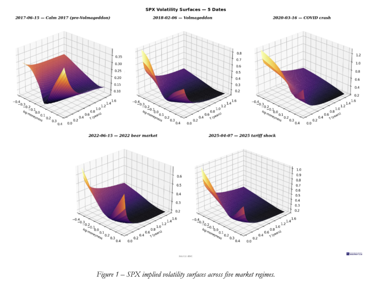
Figure 1 shows the fitted surfaces for all five dates. The differences in overall level, shape, and asymmetry are immediately apparent. In the calm 2017 regime, the surface is shallow and gently sloped: ATM implied volatility sits near 7–10% and there is only modest variation across strikes. The left wing (OTM puts) is mildly elevated above the right wing (OTM calls), and the surface is nearly flat along the maturity dimension. This picture changes dramatically during the stress episodes. The COVID crash of March 2020 produces the most extreme deformation: ATM short-term implied volatility exceeds 90%, the put wing spikes above 100%, and the entire surface lifts by roughly a factor of five to ten relative to calm conditions. Volmageddon and the 2025 tariff shock both show intermediate elevations with pronounced short-term put-wing spikes. The 2022 bear market sits somewhere in between, with a persistently elevated but more orderly surface.

What stands out across all five dates is that the short-maturity, low-strike corner of the surface, which is where crash protection is priced, is the region with the most dramatic variation across regimes. This is not surprising: it directly reflects the well-known institutional demand for downside hedging from investors who are structurally long equities.

The Volatility Smile

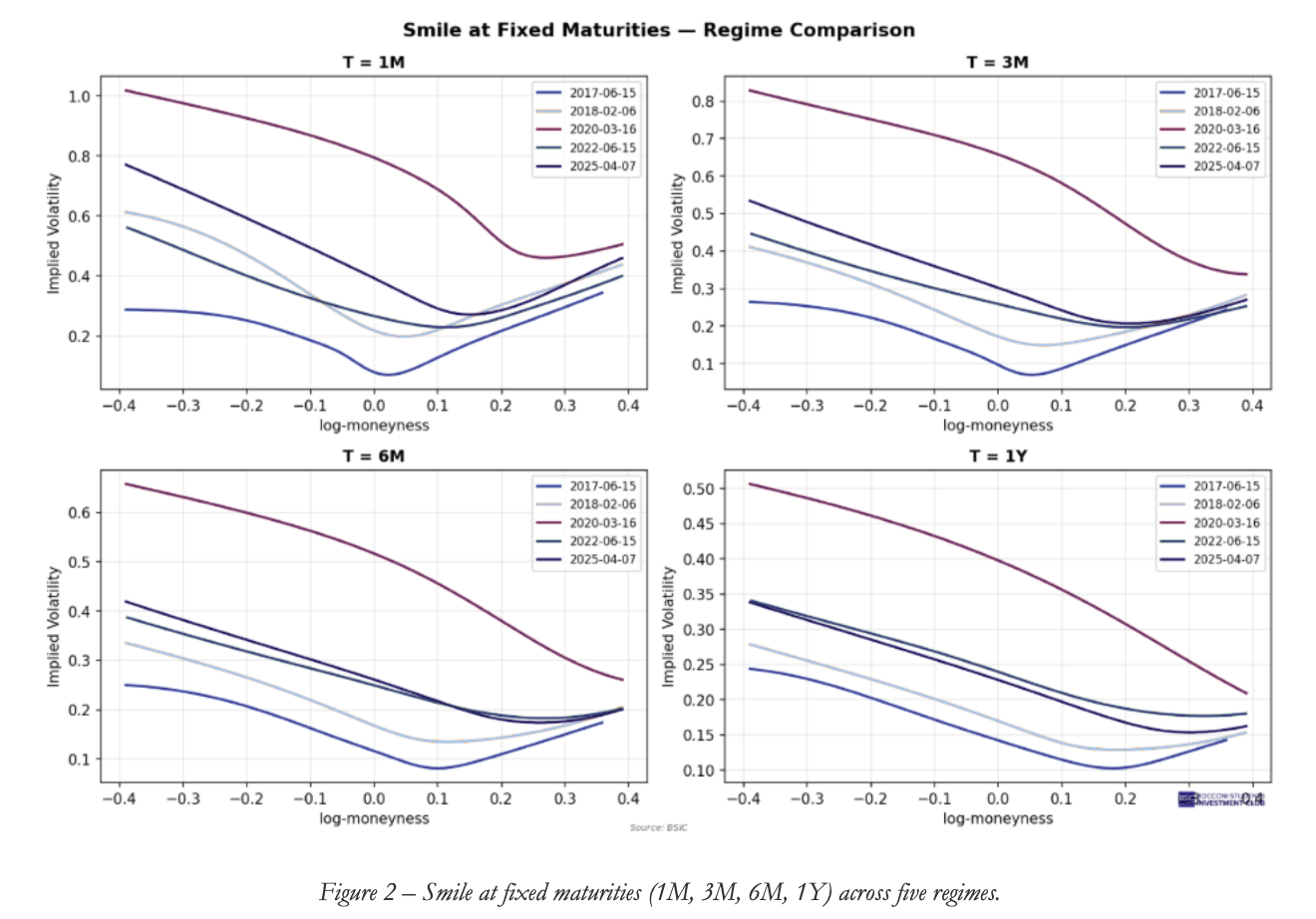
We can slice the surface vertically at fixed maturities to obtain the volatility smile, which shows how implied volatility varies across strikes for a given expiry. Figure 2 shows these slices at one month, three months, six months, and one year. In all five dates and at all maturities, the equity smile takes the form of a downward-sloping “smirk” rather than a symmetric U-shape: implied volatility is systematically higher on the put side (negative log-moneyness) than on the call side. This asymmetry is probably the most defining feature of the equity volatility surface.

The smirk is steepest at the one-month tenor. During the COVID crash the one-month IV at the deep put wing goes above 100%, while on the call side it sits around 20–25%; a spread of roughly 80 vol points. Even in the calm 2017 environment the one-month smile slopes clearly downward, though the absolute range is much narrower, going from roughly 30% on the put wing to about 5-7% on the call side. As maturity increases the smirk flattens considerably, and by the one-year tenor the differences across regimes compress and the smile becomes less steep, though it never actually becomes symmetric. This flattening with maturity is one of the most robust empirical features of the equity surface.

There are three main explanations that have been proposed for the equity skew. The first one is the leverage effect: when stock prices fall, the debt-to-equity ratio mechanically increases, raising equity volatility. This creates a negative correlation between returns and volatility which translates into higher implied volatility for low strikes. The second is jump risk: equity markets are subject to sudden large downward moves, crashes essentially, that are not captured by a log-normal diffusion. The presence of negative jump risk inflates the value of OTM puts relative to OTM calls. Bates (1991) formalised this through a jump-diffusion framework showing that the skew can be interpreted as a crash risk premium embedded in option prices. The third explanation is demand-driven: institutional investors that are structurally long equities, think pension funds, endowments, mutual funds, are natural buyers of OTM puts as portfolio insurance. This persistent net buying pressure bids up the implied volatility of the left wing. In practice all three channels operate simultaneously and the relative contribution of each one changes with market conditions. During calm periods the leverage effect and structural hedging demand are the main drivers, producing a moderate but stable skew. During crises, jump fears intensify and hedging demand becomes more urgent, which is why we see the skew steepening sharply in the COVID and Volmageddon smiles.

ATM Term Structure

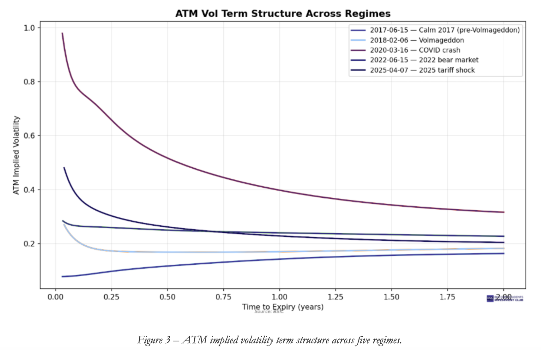
Fixing the strike at ATM ( $m = 0$ ) and reading the surface along the maturity axis gives us the ATM term structure, shown in Figu`re 3. This captures how the market’s expectation of future volatility evolves across different time horizons.

In the calm 2017 regime, the term structure is upward-sloping: short-dated ATM vol is approximately 6–7%, rising to about 15% at two years. This shape is analogous to contango in commodity futures and it reflects mean-reversion of volatility under normal conditions. Short-term realised vol is low but the market prices in the possibility of future shocks at longer horizons, which pushes the back end higher.

During crises the term structure inverts. The COVID crash shows the most extreme case: one-week ATM vol is near 100%, dropping steeply to about 30% at two years. Basically, the market is saying the current shock is transient and expects volatility to decay back toward long-run levels. The 2025 tariff shock shows a similar pattern though less extreme, with short-dated ATM vol around 50% decaying to roughly 20% at the long end. Volmageddon is different: the inversion is less pronounced, likely because the vol spike was concentrated in the VIX complex rather than in broad equity risk, and the resulting term structure is comparatively flat.

The 2022 bear market stands out for a different reason. The term structure is gently downward-sloping but neither clearly inverted nor in contango: short-dated vol of about 30% drifts toward 22–23% at the long end. This reflects a market that was pricing sustained, elevated uncertainty rather than a transient shock, which makes sense given the macroeconomic backdrop of persistent inflation and aggressive monetary tightening.

Term Structure of the Skew

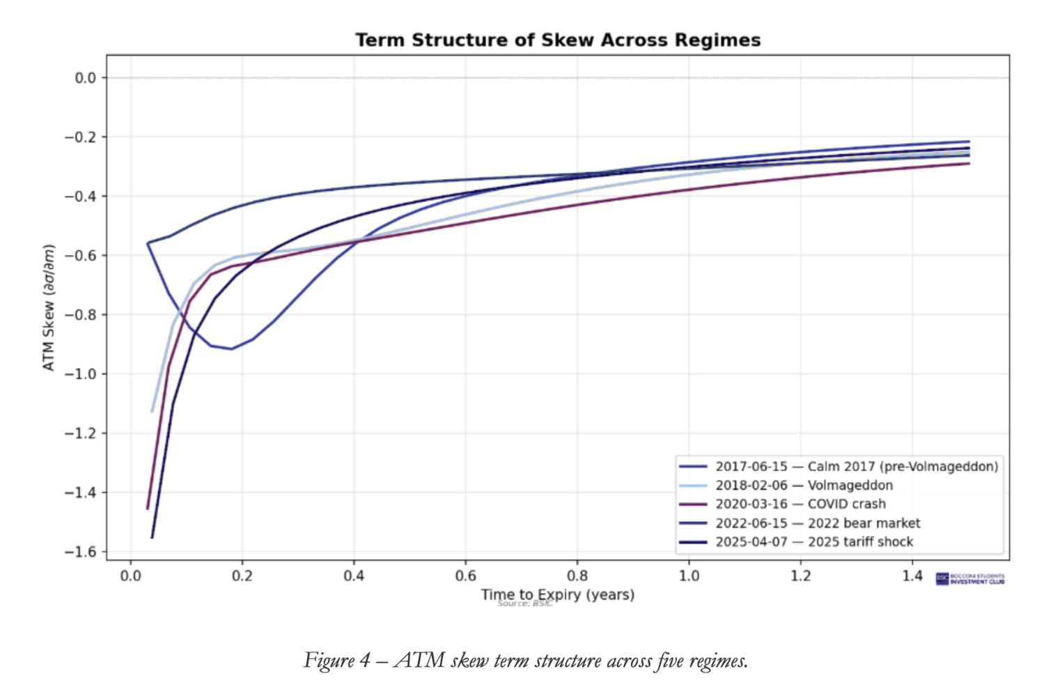
Moving to the term structure of the skew, we look at the ATM slope of the smile $\psi(\tau) = \left. \frac{\partial \sigma}{\partial m} \right|_{m=0}$ as a function of maturity. Instead of measuring the level of volatility at ATM, the skew captures the asymmetry of the surface: how fast implied volatility rises as strikes move toward the put wing.

Figure 4 shows this quantity across all five dates. The skew is negative everywhere and for every maturity, confirming that the equity smirk is a universal feature. At short maturities, below three months or so, the skew is most negative, meaning the smile is steepest. As maturity increases the skew decays toward zero in absolute value, meaning the smile flattens. This is a well-documented empirical regularity.

The shape of this decay is interesting from a modelling perspective. Under classical diffusion models like Heston (1993), the ATM skew approaches zero linearly as maturity shrinks, $\psi(\tau) \sim \tau$ as $\tau \to 0$ . However, empirical evidence from Gatheral, Jaisson and Rosenbaum (2018) has shown that the skew in equity markets blows up much faster than this: the observed behaviour is closer to $\psi(\tau) \sim \tau^{H - 1/2}$ with $H \approx 0.1$ , a power-law explosion at short maturities that standard Markovian models simply cannot reproduce. This is consistent with volatility being driven by a process rougher than standard Brownian motion, and the reader can find a more detailed treatment in the companion article on fractional Brownian motion and the rBergomi model.

Comparing across regimes we can observe two things. First, the short-end skew is most negative during crises, particularly COVID and Volmageddon, which reflects the heightened demand for crash protection and the steeper asymmetry of the risk-neutral distribution during those episodes. Second, the rate of skew decay is faster during crisis dates: beyond six months or so, all five curves converge to a relatively narrow band between roughly 0.2 and 0.35, regardless of how extreme the short end was. This convergence suggests that regime differences are concentrated at the front of the surface, while the long-end asymmetry is a more stable structural feature of equity markets, likely driven by the permanent component of the leverage effect and the baseline level of institutional hedging demand.

Taken together, the equity surface analysis reveals a market where the geometry of implied volatility is shaped by the interplay of three forces: the leverage effect linking returns to volatility, the pricing of crash and jump risk, and the supply-demand dynamics of portfolio insurance. The model-free approach allows us to capture all of these features without imposing parametric restrictions on the smile shape or on the term structure dynamics, letting the data speak directly about the risk structure embedded in SPX option prices.

FX Surface

To directly compare the FX volatility surface to that of other asset classes, we must first construct a strike-based volatility surface. FX volatility markets traditionally quote smiles in delta space because delta provides a more stable and hedging-relevant description of option moneyness than absolute strike, and because the standard smile decomposition into ATM, risk reversal, and butterfly is naturally defined at fixed deltas such as 25Δ and 10Δ.

We took the ATM volatility, 25-delta risk reversal, 25-delta butterfly, 10-delta risk reversal and converted these into pillar volatilities using: $\matrix{\sigma_{25C} & = \sigma_{ATM} + BF_{25} + \frac{1}{2}RR_{25} \\ \sigma_{25P} & = \sigma_{ATM} + BF_{25} - \frac{1}{2}RR_{25} \\ \sigma_{10C} & = \sigma_{ATM} + BF_{10} + \frac{1}{2}RR_{10} \\ \sigma_{10P} & = \sigma_{ATM} + BF_{10} - \frac{1}{2}RR_{10}}$ .

Once we had the volatility associated with each delta pillar, we used the Garman-Kohlhagen model which is the FX adaptation of Black-Scholes with domestic and foreign interest rates. For each pillar, we solve for the strike K such that the model delta matches the quoted market delta and then obtain the corresponding log-moneyness. We then interpolated these strike volatility points across maturity and moneyness to create the 3D smooth surface. Without this conversion, the FX surface would not be expressed on the same horizontal axis as other asset classes and any comparison of skew, smile or term structure would not be direct.

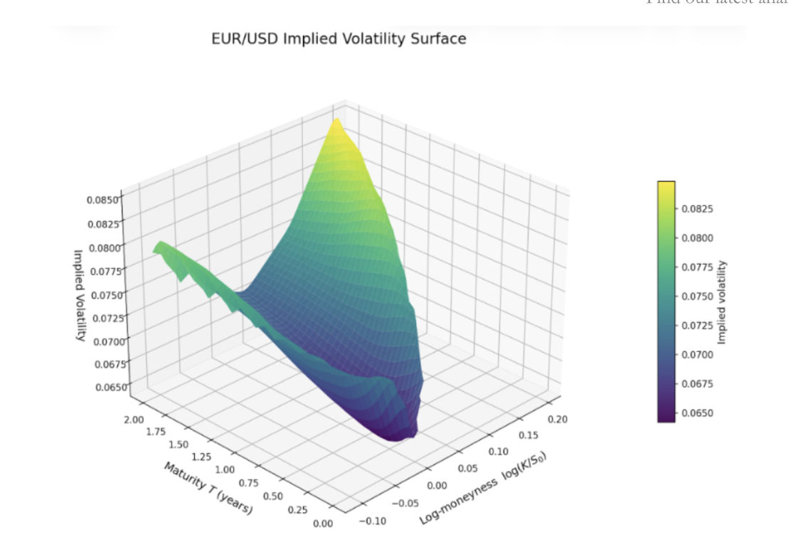
The EUR/USD surface shows a relatively low overall volatility level compared to what is typical in equities and commodities, consistent with major FX pairs generally exhibiting lower absolute implied volatility levels than equities. The smile is fairly symmetric around the centre though not perfectly so. The wings rise on both sides away from the low volatility trough, compared to equities where the left tail usually dominates. The minimum volatility sits near mildly positive log-moneyness which gives a U-shaped cross section, meaning the market prices tail risk on both sides of EUR/USD. Generally, FX term structures are strongly shaped by monetary policy expectations, interest rate differentials, macro uncertainty and event risk over longer horizons.

FX volatility surfaces are described by three components: ATM volatility, risk reversal (the difference between call and put implied volatilities at a given delta) and butterfly (average richness of the wings relative to ATM, capturing the smile). A positive or negative risk reversal gives insight to directional hedging demand and how the market prices asymmetric exchange rate risk. They tend to have more balanced tail scenarios when compared to equities due to the fact that an exchange rate is a relative price, not the value of a single corporate. FX skew is often linked to carry trades and global dollar demand – in quiet periods, carry can compress implied volatility whereas in periods of stress, unwinds can steepen skew or enrich one wing of the smile, especially if there is fear of a sharp reversal in cross-border capital flows.

Commodity Surface

Commodity volatility surfaces are structurally different from those of equities and FX, not just in shape but in the mechanisms that generate them. Unlike equities, where the leverage effect creates a persistent downside skew, commodity surfaces emerge from the interaction of four forces: physical market structure, storage and carry constraints, asymmetric hedging flows, and jump risk. These forces act directly on the forward curve and indirectly on option sensitivities, shaping delta asymmetry, gamma concentration, vega term structure, and the pricing of tail events.

This distinction is important because commodity options are typically written on futures, not spot. As a result, the relevant state variable is not spot moneyness but forward-based moneyness. For each maturity T, we define log-moneyness as $k = \ln\left(\frac{K}{F_{t,T}}\right)$ , where K is the strike price and F is the futures price corresponding to that expiry. The forward itself reflects not only the spot price but also carry conditions: $F_{t,T} = S_t e^{(r + s - y)T}$ , where r is the interest rate, s captures storage and financing costs, and y is the convenience yield. This means that the commodity volatility surface is constructed on a different economic foundation from the equity surface: both the horizontal axis and the interpretation of “at-the-money” are tied to the futures curve rather than the spot level.

In practical terms, each point on the surface is the implied volatility that solves the Black futures option formula for a given strike and maturity. The surface therefore should not be viewed as a purely statistical forecast of future volatility. It is better understood as the market-clearing price of convexity, hedging pressure, and tail risk at each forward moneyness and expiry. Put differently, the commodity surface is where the economics of storage, inventory scarcity, and jump exposure are translated into option Greeks.

Why the Greeks are different in commodities

The first distinction is that delta is naturally defined with respect to the forward or futures contract rather than spot. Since the forward level already embeds carry, storage, and convenience yield, the location of the at-the-money strike shifts with the shape of the curve. In a backwardated market, the forward is below spot, while in contango it is above spot. As a result, the apparent skew of the surface is partly a function of how the forward curve maps strikes into moneyness. Commodity skew is therefore not simply “left-tail fear” in the equity sense; it is often a combined reflection of forward curve shape, hedging demand, and the distribution of physical shocks.

The second distinction concerns theta. In equities, theta is often interpreted primarily as time decay. In commodities, theta is more naturally thought of as time decay interacting with carry. Because the forward depends on storage costs and convenience yield, the passage of time changes not only the option’s remaining maturity but also the economics of the underlying futures position. A high convenience yield, for example, lowers the forward relative to spot and changes where gamma is concentrated around the money. Theta in commodity options is therefore partly a carry phenomenon and not just a mechanical erosion of option premium.

The third distinction is market microstructure. Liquidity in commodity options is often concentrated in the front month, especially in oil and other physically sensitive contracts. This has immediate Greek implications: gamma is concentrated in short-dated maturities, front-end vega dominates risk management, and implied volatility term structures can become very steep. When inventories are tight or delivery constraints matter, short-dated options absorb the bulk of market uncertainty, producing unstable gamma and rapid repricing of near-term tails.

The four forces behind the commodity surface

The first force is physical market structure, especially the distinction between contango and backwardation. Backwardation usually signals scarcity of the physical commodity today, while contango is more consistent with abundant supply and positive carrying costs. In periods of scarcity, the front of the curve becomes highly sensitive to even small supply or demand shocks. This translates into high short-dated implied volatility and, often, a downward-sloping term structure of volatility. In Greek terms, the market is pricing gamma: when near-term supply is tight, a small fundamental shock can create a disproportionately large move in the prompt futures contract. The result is elevated front-month gamma, fast theta decay, and a front-heavy vega profile.

The second force is storage, convenience yield, and inventories. Inventories are central because they determine how easily the physical market can absorb shocks. When inventories are high, the market has a buffer; supply and demand imbalances can be smoothed, and price responses are more linear. When inventories are low, that buffer disappears and the supply curve becomes much more convex. Under those conditions, small shocks can produce outsized price moves. This matters directly for the surface: low inventories tend to raise implied volatility, especially at the front end, and can create severe distortions in nearby maturities. In economic terms, inventories determine how nonlinear the price response is to shocks. In option terms, that is exactly what gamma pricing captures. This is why episodes of binding storage constraints, such as the dislocation in oil markets in April 2020, produce not merely high volatility but extreme front-end convexity.

The third force is asymmetric hedger positioning. In equity markets, skew is relatively stable because the underlying mechanism is structural: a falling equity price mechanically raises leverage and increases risk. Commodity skew is more flow-driven. In oil, producer hedging can generate strong demand for downside protection, which supports put implied volatility. At the same time, the market remains exposed to upside supply shocks, such as geopolitical disruptions or weather events, which can make call wings expensive as well. The result is that the skew in oil can be unstable, flatter than equity skew in some periods and even tilted toward calls in others. Gold is different. Its options market is typically driven by more balanced macro hedging flows, reserve demand, and broader uncertainty over rates, inflation, and the U.S. dollar. As a result, gold tends to exhibit a more symmetric smile than crude oil or equities. In Greek language, commodity skew is best interpreted as a flow equilibrium rather than a leverage effect. Dealer positioning, customer hedging demand, and inventory-related uncertainty all influence where delta risk becomes expensive.

The fourth force is jump risk. Commodity prices are especially vulnerable to discrete shocks: geopolitical events, production outages, weather disruptions, transportation bottlenecks, policy interventions, and sudden demand collapses. A diffusion-only view of price dynamics therefore misses a major part of the economic reality. These jump risks are reflected in rich wing volatilities and pronounced smile curvature, especially in short-dated contracts where uncertainty is immediate. Deep out-of-the-money options are not only insurance against large moves; they are instruments for pricing non-hedgeable discontinuities. In Greek terms, jumps make delta hedging unstable and increase the value of tail gamma and vega convexity. This is one reason why commodity smiles often remain pronounced even when realized day-to-day volatility looks contained.

Oil: a surface shaped by inventories, storage, and jump risk

The crude oil surface is the clearest illustration of how physical market structure feeds into option pricing. Relative to equities and FX, oil typically shows three features. First, implied volatility is often highest at the front end of the curve. Second, the term structure of volatility can slope sharply downward when inventories are low or supply conditions are stressed. Third, the skew is less stable than in equities: it may reflect put demand from producers in some periods, but upside call premia can become equally important when the dominant risk is a supply interruption.

These features can be read directly through the Greeks. Elevated prompt volatility means that front-month gamma is expensive. Short-dated oil options are highly sensitive because the underlying contract is exposed to immediate inventory and delivery conditions. That same concentration of risk causes rapid theta decay, since a large share of the option premium is compensation for short-lived but intense uncertainty. Wing options, meanwhile, price the possibility of discrete events, so tail gamma and smile curvature are often elevated relative to smoother asset classes.

The economic drivers behind this shape are intuitive. When inventories are comfortable, the oil market can absorb shocks through storage drawdowns or replenishment, and price responses are more moderate. When inventories are low, the market loses that flexibility. The prompt contract then becomes the focal point of adjustment, and volatility rises sharply at the front of the surface. Storage constraints intensify this effect, because once storage binds, prices no longer respond linearly to fundamentals. The April 2020 episode is the extreme example: as storage capacity approached its limit, the prompt oil contract experienced a breakdown of normal price relationships, and the market effectively repriced near-term gamma at exceptional levels. The surface in such episodes is not simply “high vol”; it is a map of acute physical stress.

Oil skew is also distinctive because it is not pinned down by a single structural mechanism. Producer hedging can lift put demand, but geopolitical risks and supply disruptions can lift call demand as well. For that reason, the oil smile often contains more information than the oil skew alone. It reflects a market that is pricing both downside growth shocks and upside scarcity shocks at the same time.

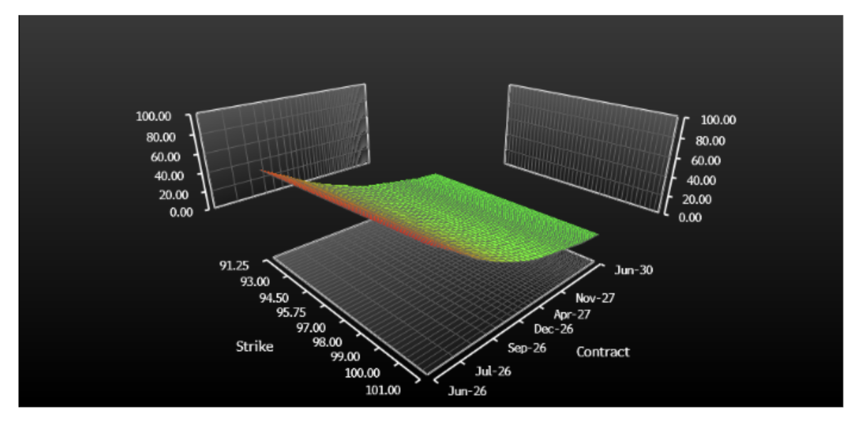
The volatility surfaces for oil and gold observed on April 14 illustrate how differently commodity markets encode risk through option prices. The oil surface appears relatively smooth across strikes but exhibits a pronounced structure across maturities, with implied volatility elevated in the front contracts and declining steadily along the curve. This downward-sloping term structure indicates that the market is primarily pricing short-term uncertainty rather than long-term dispersion. The lack of extreme curvature across strikes suggests that skew is not structurally driven, as in equities, but instead reflects more transient factors such as hedging flows and jump risk. In Greek terms, this corresponds to a concentration of gamma in the front end of the curve, where prices are highly sensitive to near-term shocks, and a vega profile that is similarly front-loaded. Economically, this is consistent with a market where inventory levels and physical constraints dominate, making prices highly responsive to immediate supply and demand imbalances.

Gold: a surface driven more by macro uncertainty than physical scarcity

Gold offers a useful contrast because its surface is typically less dominated by immediate physical bottlenecks. While gold is of course a commodity, its option market behaves more like a macro-financial market than a storage-constrained industrial market. Gold prices are strongly influenced by real rates, inflation expectations, U.S. dollar dynamics, and safe-haven demand. As a result, its volatility surface is usually flatter in term structure and more symmetric in smile shape than crude oil.

From a Greek perspective, gold tends to price vega more consistently across maturities than oil does. The front end can still react sharply to macro events such as central bank surprises or sudden risk-off episodes, but the distribution of uncertainty is not usually dominated by near-term delivery stress. This makes gamma spikes less extreme and the term structure of implied volatility more stable. Delta skew is also more balanced, reflecting the fact that gold is used both as an inflation hedge and as a defensive asset during financial stress. Unlike equities, where downside fear dominates, or oil, where physical scarcity can make upside tails especially important, gold often displays a more symmetric market price of tail risk.

This difference can be summarized neatly: oil often prices the convexity of supply, while gold more often prices macro uncertainty. Oil’s surface is shaped by inventories, convenience yield, and delivery constraints. Gold’s surface is shaped more by rates, currency conditions, and broad risk sentiment. That is why gold usually carries a smoother vega term structure and a more regular smile, whereas oil is more prone to abrupt front-end distortions and unstable skew.

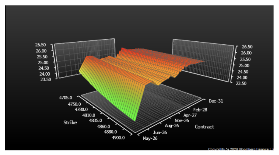
By contrast, the gold volatility surface is flatter across maturities and exhibits a more pronounced and symmetric smile across strikes. The relatively stable term structure suggests that uncertainty is not concentrated in the near term but persists across horizons, reflecting the influence of macroeconomic factors such as interest rates, inflation expectations, and currency movements. The clearer curvature across strikes indicates that both upside and downside tail risks are being priced more evenly, resulting in a balanced smile rather than a directional skew. From a Greeks perspective, this implies a more evenly distributed vega exposure across maturities and less extreme gamma concentration in the front end. Unlike oil, where physical scarcity and storage constraints drive nonlinear price responses, gold behaves more like a macro-financial asset, with its volatility surface shaped by broad, persistent uncertainty rather than immediate physical shocks.

Technical interpretation and model intuition

These empirical patterns also align with standard commodity option theory. Mean reversion in commodity prices tends to dampen long-dated variance, which helps explain why back-end implied volatilities are often lower and less reactive than the front end. Seasonality can make volatility maturity-dependent, especially in energy and agricultural contracts, producing predictable variations in theta and vega across the curve. Jump-diffusion logic explains why short-dated wings remain expensive even when realized volatility is temporarily subdued: the market assigns value to protection against discontinuous shocks. Two-factor commodity models, such as those that treat spot and convenience yield jointly, are especially useful conceptually because they show how convenience yield operates as a state variable linking inventories, the forward curve, and ultimately the shape of the volatility surface.

Conclusion

Read together, these three dimensions reveal the distinct risk architecture of each market: equity surfaces encode leverage and crash risk, FX surfaces reflect bilateral macro uncertainty, commodity surfaces map the economics of physical supply and hedging flows. The differences are not artefacts of model choice: they are genuine features of how each market prices risk.

Neural Network Calibration

Motivation

Having compared volatility surfaces across equities, foreign exchange, and commodities, the final question is whether such surfaces can be mapped efficiently into a parametric model representation. In a standard Heston calibration, this requires solving a numerical optimisation problem separately for each date and each asset, which is computationally expensive and can become unstable when the parameters are only weakly identified by the observed surface. A natural alternative is a neural network: train the model once to learn the inverse mapping from an implied-volatility surface to the corresponding Heston parameter vector, and then use it to produce near-instantaneous calibrations.

This is useful for two reasons. First, it has clear practical value. If successful, neural calibration would provide a much faster tool for large-scale empirical work, real-time monitoring, and repeated scenario analysis. Second, a successful network would suggest that the information contained in the surface is sufficiently structured for a statistical learning model to recover stable parametric factors. The neural-network experiment is therefore both a computational extension and a diagnostic test of how well a low-dimensional stochastic-volatility model can represent observed option surfaces.

In this setting, the neural network is used to solve the inverse calibration problem: given an observed implied-volatility surface, estimate the Heston parameter vector that would reproduce it. Because the true Heston parameters are not observed in market data, supervised learning must be based on synthetic data generated from known parameter vectors. For that reason, the network was trained on a synthetic bootstrap distribution constructed from QuantLib calibrations and real SPX surface variation. Its practical purpose is to replace slow iterative calibration with near-instantaneous prediction, while its scientific purpose is to test whether real market surfaces contain enough stable information for a low-dimensional parametric model to be recovered reliably.

Results

To implement this, we first calibrated a Heston model in QuantLib across multiple SPX option dates, taking every Wednesday in 2023 and using the resulting calibrated parameter vectors as benchmark estimates. The last 10 dates were held out as an out-of-sample test set. For the remaining in-sample dates, we paired each calibrated parameter vector with its corresponding implied-volatility surface, reduced the surface dimension using PCA, and modelled the joint distribution of transformed Heston parameters and surface-PC coordinates with a multivariate normal distribution. Sampling from this joint distribution produced a large synthetic dataset of Heston parameter/surface pairs, on which the neural network was trained to learn the inverse mapping from surface to parameters.

The model was then evaluated in three stages: first on held-out synthetic data, then on in-sample real market surfaces, and finally on out-of-sample real market surfaces. After the neural network predicted a parameter vector, we repriced the corresponding Heston surface and compared it with the observed market surface using implied-volatility RMSE. This surface-level metric is the economically relevant measure of calibration quality, since a parameter estimate is only useful insofar as it reproduces the observed option surface.

The results show a clear contrast between synthetic and real-market performance. On the synthetic validation set, the neural network learned the inverse Heston map well, with all five parameters achieving strong out-of-sample performance and R² values between 0.90 and 0.98. This confirms that the network successfully learned the inverse mapping on the synthetic bootstrap distribution. On real SPX surfaces, the network also produced reasonably good implied-volatility surface reconstructions: mean IV RMSE was approximately 0.20 versus 0.185 for QuantLib in-sample, and 0.211 versus 0.190 out-of-sample. The error gap remained stable across the in-sample/out-of-sample boundary, indicating that the network generated consistently reasonable surface reconstructions.

However, this surface-level success did not translate into reliable parameter recovery. Although the network performed well on synthetic validation data, its real-market parameter predictions were poor and, after clipping to admissible bounds, collapsed toward an almost constant parameter vector across dates. The relatively good surface RMSE therefore does not imply successful real-market inversion. Rather, it suggests that a near-constant Heston parameter vector can still generate a generic SPX-like volatility surface that lies tolerably close to many observed market surfaces. The most likely explanation is the weak identifiability of Heston parameters: multiple parameter combinations can produce very similar volatility surfaces, so the network appears to regress toward a stable prior-like parameter vector rather than recover the date-specific QuantLib calibration.

Taken together, these findings suggest that neural calibration works very well within the synthetic Heston distribution on which it is trained, but generalises only weakly at the parameter level to real market surfaces. Its main success is therefore computational and surface-level rather than structural: it can reconstruct a plausible surface quickly, but it does not reliably recover unique date-specific Heston parameters from observed SPX option data.

References

[1] Sheldon Natenberg, “Option Volatility and Pricing: Advanced Trading Strategies and Techniques”, 2nd ed., McGraw-Hill, 1994.

[2] Paride Lauretti, Riccardo Favazza, “Implied Volatility Surface Modelling: A Quantitative Framework for Construction, Calibration and Risk Management”, Bocconi Students Investment Club, December 2025.

Published by BSIC on 19 April 202619 April 2026

0 Comments

Leave a Reply Cancel reply

Attention Factors

Market Recap 19/04/2026

Understanding Convexity Bias in STIR Futures Markets