Modelling Swap Spreads

Download PDF

Introduction

Swap spreads, which measure the difference between the fixed rate on a swap and the yield on a Treasury bond of the same maturity, have often been negative in recent years, particularly in the wake of the financial crisis of 2008. This phenomenon has puzzled market participants, as negative swap spreads imply that investors are willing to accept lower yields on swaps than on Treasuries. In this article, we review the literature on swap spreads and develop a model that explains swap spreads with different factors related to supply and demand for swaps and Treasuries, liquidity risk, credit risk, and regulatory changes.

Interest Rates Swaps and Swap Spreads

An interest rates swap (IRS) is an agreement to exchange different types of cash flows. The plain-vanilla IRS is based on a fixed leg, which pays a constant interest rate on a notional amount, and a floating leg, which is instead anchored to a floating rate such as the 3M LIBOR or SOFR. The party that receives the fixed interest rate is called receiver, while the other party is the payer. Clearly, the payer believes that rates are going to rise, or more precisely the duration of the payer’s position is negative. Moreover, convexity for the payer is negative as well.

Figure 1: The structure of a plain-vanilla IRS
Source: Bocconi Students Investment Club

In order to price a swap, we assume that the present values of the two legs are equal at inception, otherwise one the parties would not enter the trade. The swap rate is the value which satisfies this equality, and it can be derived by solving the following formula for a semi-annual swap:

where are the zero-coupon rates for the semi-annual maturities. For the floating leg, the present value is at par, since the coupon is itself the market rate on a coupon date. However, accrued interest should be taken into account when computing the present value on a non-coupon date. The fixed rate on an IRS can be thought of as weighted average of forward short-term rates, therefore trading swaps entails having a view on short-term rates with respect to market expectations.

IRS are among the most liquid financial products, with a current Gross Notional Outstanding of $289trn, $116trn of which is USD-based. The high liquidity of swaps is primarily due to the flexibility of their OTC nature and their wide range of applications, namely, interest rate risk management. For instance, consider a company that issues floating rate debt: the company can enter a swap as a fixed payer to convert its interest rates exposure from floating to fixed, by receiving the floating leg and using it to pay back its bondholders. The same operation can be carried out by a bond investor to convert fixed to floating, also known as asset swapping.

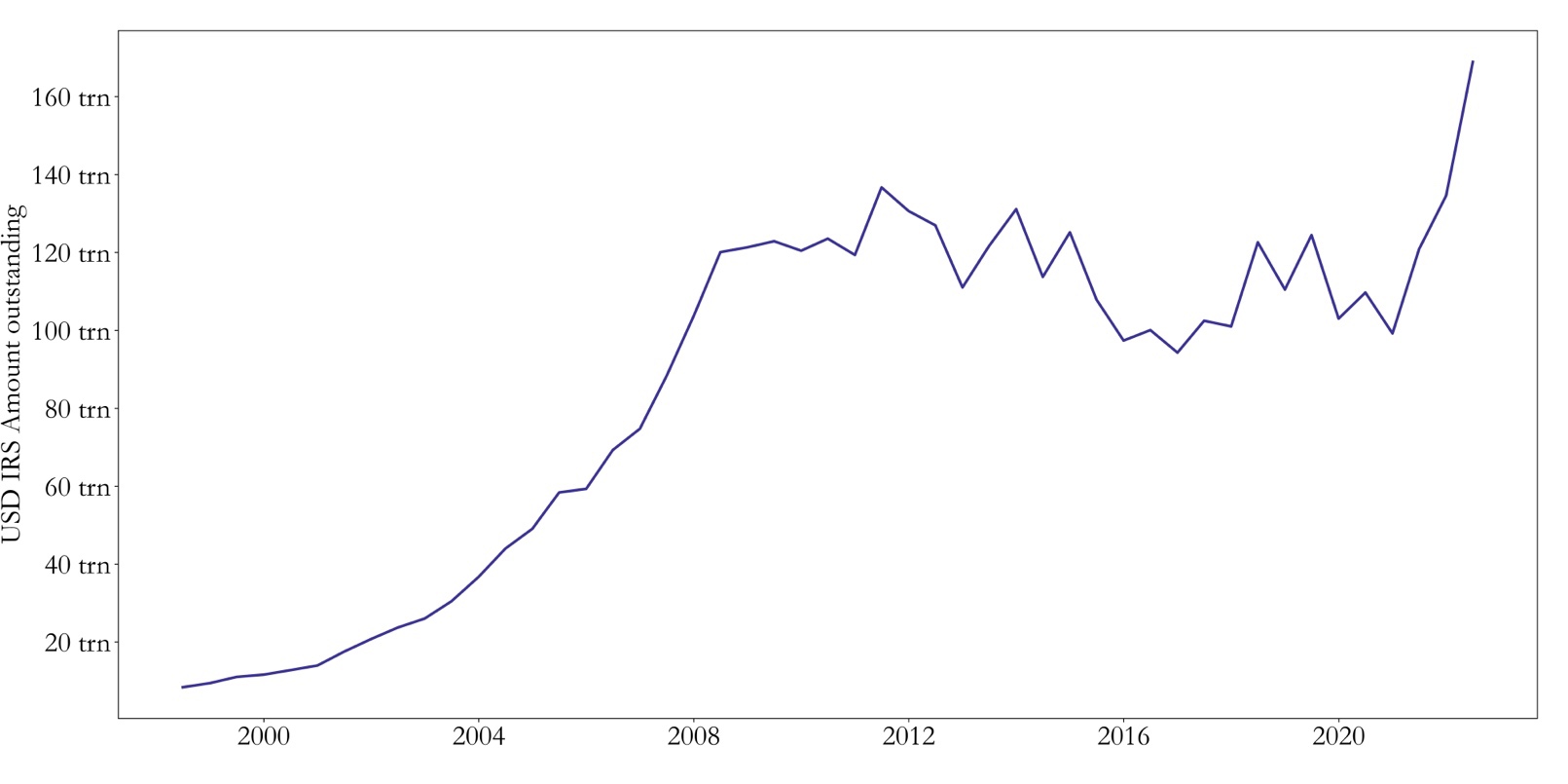
Figure 2: Outstanding USD IRS
Source: BIS, Bocconi Students Investment Club

As with other derivatives products, the OTC nature of swaps has both advantages and disadvantages – the former being higher flexibility and the absence of an up-front notional amount, and the latter being counterparty risk. In order to reduce the counterparty risk, swaps must adhere to some principles specified by ISDA (International Swap Dealer Association). Starting from 2008, the swap market has been affected by several regulatory reforms, the main one being Dodd-Frank Act in 2013, which imposed mandatory trading reporting and clearing.

Swap spreads are defined as the maturity-matched spreads between swap rates and Treasury yields. Swap spreads based on LIBOR could then be used to express a view on the systemic risk of the banking system, represented by the LIBOR-GC repo spread. However, there are two problems: (1) LIBOR is subject to survivorship bias, because if an individual bank has its credit downgraded, it gets delisted from the LIBOR panel, therefore not affecting the LIBOR rate significantly; (2) LIBOR-GC repo spread was not found to be a statistically significant driver of swap spreads by Cortes (2003) and Kobor (2005). We rather observe that swap spreads are primarily driven by supply-and-demand dynamics, uncertainty, and expectations on the economic outlook.

Finally, we note that the transition from LIBOR to SOFR, starting in 2018, had significant implications for the swap market and the potential arbitrage opportunities. As LIBOR was phased out, the potential mismatch between LIBOR-based swaps and new SOFR-based derivatives led to a brief decline in liquidity and widening of spreads. Market participants needed to adjust their strategies and re-evaluate their pricing models, especially what concerns the term structure, to incorporate the new SOFR benchmark. For an analysis on the LIBOR-SOFR transition, please refer to this series of BSIC articles.

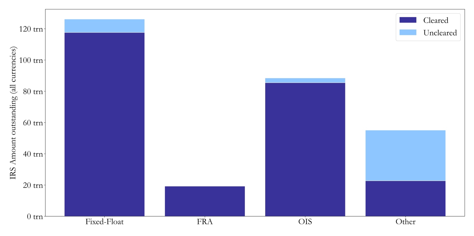
Figure 3: Outstanding IRS (all currencies) by type
Source: CFTC, Bocconi Students Investment Club

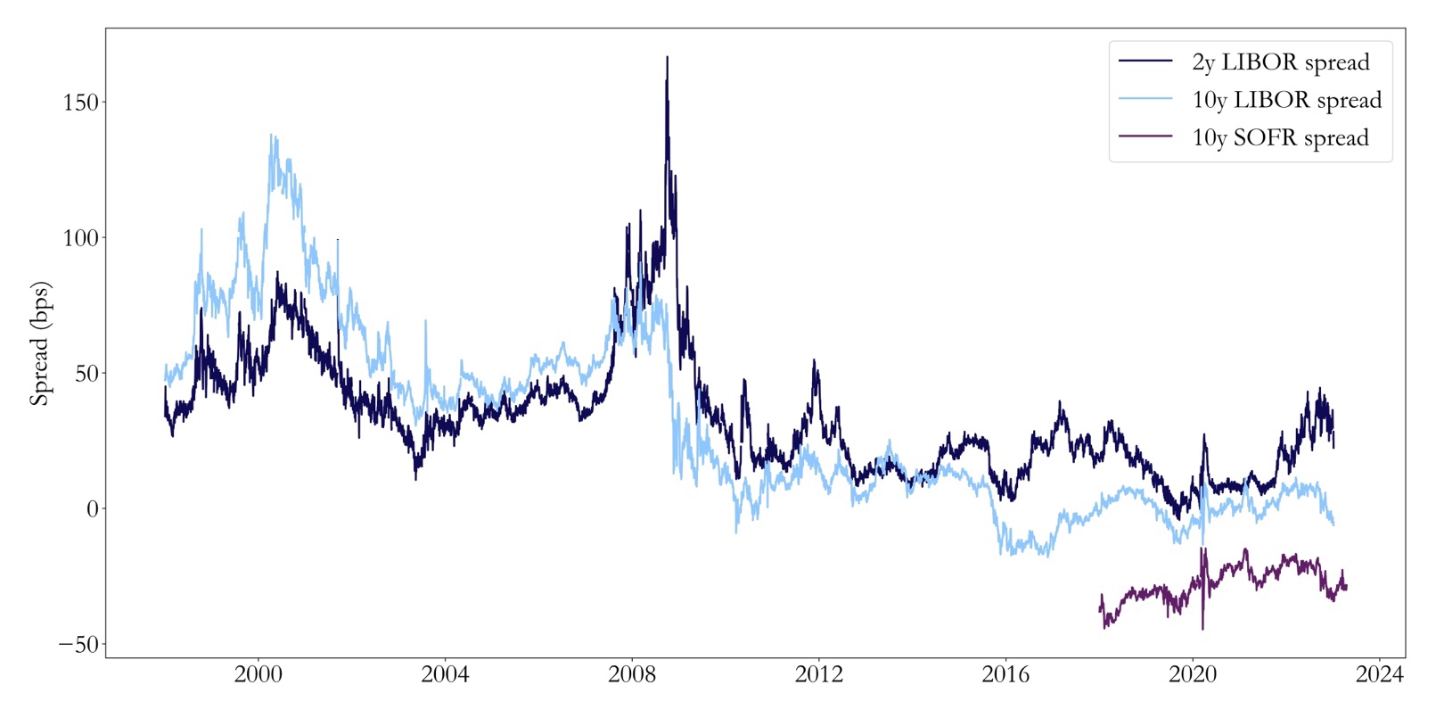
Figure 4: 2y LIBOR, 10y LIBOR, 10y SOFR swap spreads
Source: Bloomberg, Bocconi Students Investment Club

Swap Spread Trade Mechanics

In this section we analyse the swap spread trade mechanics, emphasizing the financing costs of both legs of the trades. For the sake of simplicity, we will just consider the trade with a long Treasury position for the cash leg and pay-fixed for the swap leg. The trade is from the point of view of a dealer, but it can be easily extended to a dealer’s client (e.g. hedge fund) by considering the dealer-client transaction. We also assume that the dealer is bound to finance the cash leg through the repo market, which is the topic of this series of BSIC articles.

The cash leg is structured as follows:

• The dealer buys a Treasury security (UST) and uses it as a collateral to borrow from the repo market at the general collateral repo rate, or at a lower rate if the UST is trading on special (see here).
• Since the repo applies a haircut on the amount being borrowed by the dealer, the dealer needs to borrow the haircut on the unsecured money funding at an overnight indexed swap (OIS) rate.

The swap leg is structured as follows:

• The dealer enters a pay-fixed swap with the same maturity as the UST, receiving a short-term interest rate.
• Since the swap is centrally cleared, the dealer needs to post initial and variation margins, which it borrows from the unsecured funding market at an OIS rate.

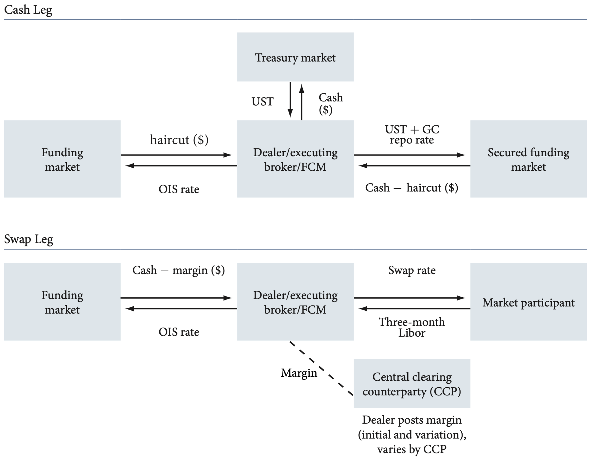
Figure 5: Swap trade mechanics overview
Source: Boyarchenko (2018), edited by Bocconi Students Investment Club

As it is clear from the scheme above, the structure of a swap spread trade is quite complex and it has non-trivial consequences on the dealer’s balance sheet cost, which will be further analysed. Finally, we can observe that the haircut and the margin play a similar role from a financing point of view.

We conclude by noting that a positive spread on a LIBOR swap does not represent a no-arbitrage failure since 3-month LIBOR surpasses the secured financing rate for Treasuries. This is because receiving fixed on a LIBOR swap and shorting Treasuries can generate negative cashflows if the LIBOR–OIS short-rate differential is sufficiently large (or LIBOR-GC collateral). However, assuming that LIBOR always surpasses OIS, a negative LIBOR swap spread violates the no-arbitrage principle. In this case, paying fixed on a LIBOR swap and taking a long position in Treasuries creates a zero-cost portfolio with strictly positive cashflows in all possible scenarios across 10-30 years (where the negative swap spread is deeper and more persistent).

To whoever postulates that this risk-free trade should be arbitraged out, the literature posits that the risk of convergence is a significant factor affecting long-dated swap spreads. Profiting from these spreads not only requires a considerable amount of capital, but it also involves risk for investors. Any future shocks to the demand or supply of the market could cause the spreads to widen unexpectedly, leading to short-term losses and increased margin requirements for these intermediaries. As a result, they demand compensation for the risk they bear in the event of supply-demand imbalances, which ultimately raises the magnitude of swap spreads, particularly for longer maturities.

The Drivers of Swap Spreads

Since there is compelling evidence suggesting a significant change in market demand occurred towards the end of 2008, leading to a shift from a preference for paying the fixed swap rate to a preference for receiving it, we will proceed to a description of the main players transacting in the long-dated IRS market, as discussed in the Treasury Borrowing Advisory Committee’s recent report on the swap market.

First of all, insurers and pension funds consider swaps paramount to manage their exposure to interest rate risk. They typically receive the fixed swap rate on net, using swaps to add duration, as the duration of their liabilities exceeds that of their on-balance sheet assets (as discussed in a recent BSIC article). As we will discuss below, when pensions become more underfunded, their desire to receive fixed increases. Insurers and pensions enter into additional receive-fixed swaps when long-term rates fall, to dynamically manage their interest-rate exposure.

On the other hand, commercial banks typically used receive fixed on net to offset their pre-existing exposures to declining interest rates of the recent decade, as they borrowed short-term and lend long-term, and are generally hurt by declining interest rates because their loans reprice more quickly than their deposits. For this purpose, an interesting concept is the one of deposit betas, as analysed by the New York Fed in Liberty Street Economics. Deposit betas refer to the extent to which changes in the federal funds rate affect deposit rates, and they can be used to measure the pass-through of monetary policy to the deposit market. Specifically, the deposit beta is the fraction of a change in the fed funds rate that is transmitted to the deposit rate. In general, deposit rates tend to adjust to changes in the fed funds rate with some lag, especially during an upward rate cycle. For instance, during 2022 Q4, when the Fed funds rate hovered around 3.7%, the interest-bearing deposit rate reached only 1.4%. However, the speed of adjustment has been faster in the current rate-hiking cycle, which could be attributed to the more rapid pace of interest rate increases.

For what concerns non-financial corporations, they typically receive fixed on net to convert fixed-rate debt issues into synthetic floating-rate funding. We also point out that SIFMA (i.e. Securities Industry and Financial Markets Association) indicates that the average maturity of newly issued bonds has increased significantly over the years, ranging from 7.3 years in 2000 to 18.5 years in 2020. As stated prior, this results in further hedging through long-dated IRS.

Relative-value mortgage investors pay the fixed swap rate on net to hedge mortgage-backed securities (MBS) with swaps instead of Treasuries for regulatory and accounting reasons, and because swaps have been a more effective hedge. When long-term rates fall, expected mortgage prepayments rise, causing MBS duration to decline. This prompts mortgage investors to enter receive-fixed swaps to reduce the size of their pay-fixed hedge positions. Mortgage servicers earn a stream of fees that makes their exposure similar to the holder of an interest-only MBS strip, which typically has a negative duration. Since the strips are negatively convex just like MBS, servicers tend to increase their receive-fixed positions when rates fall.

Finally, swaps are utilized by fixed-income money managers to modify the duration of their portfolios, and they usually hold cash bonds and prefer pay-fixed swap positions to achieve their duration objectives. Moreover, convexity-driven hedging usually results in a rise in the net demand to receive fixed when interest rates decrease.

Prior to the Global Financial Crisis (GFC), hedged mortgage investors held a significant position in the swap market, resulting in a net demand to pay fixed rates. On the supply side, dealers and fixed-income hedge funds accommodated this demand by adopting a long swap spreads strategy, whereby they received the fixed swap rate and simultaneously took offsetting short positions in Treasuries (Duarte et al. 2006). This approach proved popular and led to many dealers and hedge funds having substantial long positions in this swap spread trade, as demonstrated by the 1998 Long-Term Capital Management crisis reports (Lowenstein, 2000). With hedged mortgage investors retreating from the market in 2008, there was a significant shift in demand swinging from a desire to pay fixed to one to receive fixed.

Swap spreads are found to have a long-term cointegration relation with budget balance expectations (Cortes, 2003). High budget balance expectations imply low government bond issuance expectations – its tax revenue is high – which means low supply of Treasuries and low yields for specific sectors of the yield curve. This in turn leads swap spreads to widen. Conversely, swap spreads tend to decrease when budget balance expectations are negative.

Periods of high uncertainty have historically been associated with “flights to quality”, that is investors rushing into safe assets like US Treasuries. During these periods swap spreads are set to widen, due to the decrease in Treasury yields. We proxy for uncertainty by looking at future volatility implied by the equity markets (VIX) or risk aversion indices such as Bekaert-Engstrom-Xu Uncertainty Index (BEX Index). Moreover, during periods of uncertainty most securities command a higher liquidity risk premium with respect to Treasuries, driving swap spreads higher. On-the-run/off-the-run spread, that is the spread between the on-the-run Treasury and the first off-the-run Treasury, can be used to proxy for liquidity.

Finally, swap spreads tend to tighten when the yield curve steepens. This relationship has two main explanations: (1) demand for receiving fixed increases, since fixed-rate bond issuers are more prone to swap to floating, and commercial banks are less concerned about hedging their short-term variable deposits, thereby reducing their fixed-payer exposure, (2) a steep curve environment is associated with expectations of future economic growth, which also means that the risk perceived for the financial system is low (see above LIBOR-GC spread).

The Case for Negative Spreads

Following the default of Lehman Brothers in September 2008, the 30-year swap spread experienced a sharp decline and turned negative. The 10-year swap turned negative in the Fall of 2015. These occurrences represent a theoretical arbitrage opportunity and a pricing anomaly that can be explained in detail (see above). However, in comparison to other financial crises, this negative swap spread has remained remarkably persistent over time.

Boyarchenko (2018) provides an explanation for negative swap spreads based on trading costs, regulatory requirements, and limits to arbitrage. As previously explained, negative swap spreads would offer a pure “carry” arbitrage by just entering a spread widening trade. However, this statement is rejected when considering that interest rates are not the only risk factor at play. Regulatory changes can explain why swap spreads have been in negative territory for the past years: dealers’ return on equity (ROE) for entering a widening spread trade has been vastly affected by capital regulations since the fall of 2015, the main one being supplementary leverage ratio (SLR), i.e. the amount of common equity capital relative to the total leverage exposure. Higher leverage requirements have decreased the swap spread at which dealers can earn a given ROE. We can think about this level of swap spread as being the “arbitrage spread” or the “break-even spread” for a certain trade, once we fix the SLR, the financing costs, and the targeted ROE. Finally, it is important to note that regulatory requirements are not by themselves the cause of negative swap spreads, but they rather act by making market participants less willing to enter spread trades across linked markets, thus leading to prolonged market dislocations (see literature on intermediary asset pricing).

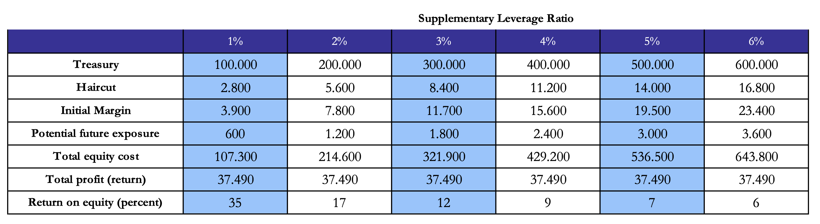
Figure 6: Swap spread returns given the Supplementary Leverage Ratio (SLR)
Source: Boyarchenko (2018), Bocconi Students Investment Club

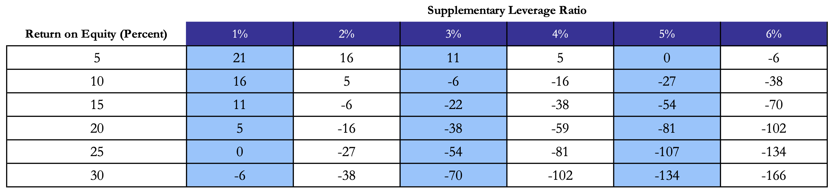
Figure 7: Return on Equity on a swap spread position given the Supplementary Leverage Ratio (SLR)
Source: Boyarchenko (2018), Bocconi Students Investment Club

Klinger (2019) presents an alternative explanation for negative swap spreads based on demand-side factors. The model centers on the concept of pension plans with insufficient funding for their long-term liabilities, which in turn prompts them to pursue duration hedging via the fixed rate in long-maturity IRSs. These pension funds have obligations in the form of unfunded pension claims and investments in a diversified portfolio of assets with varying durations and, to balance their asset-liability durations, they can either invest in long-term bonds or receive fixed payments in an IRS with a long maturity. Their theory posits that underfunded pension plans prefer hedging their duration risks by entering into IRSs instead of purchasing Treasuries, which may not be feasible considering their funding status. This preference for using IRSs to hedge duration risk arises due to their relatively lower margin requirements compared to the outright investment required for government bonds. The same phenomenon spreads its evidence in the English, Dutch and Japanese market, where the size of pension funds involved in financial transactions are preponderant. The underfunded ratio (UFR) is shown below:

Our Analysis

Our empirical contributions are closely related to the work of Cortes, 2003 and Kobor, 2005, in that we assess the drivers of swap spreads from a statistical point of view by performing a regression analysis. We construct a panel of monthly data made of several covariates and two swap spreads, 10y LIBOR and 10y SOFR. The covariates are:

• Slope of the yield curve, that is the spread between 10y Treasury and 2y Treasury (FRED)*;
• VIX index (FRED)*;
• MOVE index (Bloomberg);
• Bekaert-Engstrom-Xu Uncertainty Index (Bekaert-Engstrom-Xu website);
• Bloomberg US MBS Index Statistics Modified Adjusted Duration (Bloomberg)*;
• Treasury securities outstanding, total marketable (Bloomberg)*;
• United States Federal Government total surplus or deficit (Bloomberg)*;
• Milliman 100 Pension Funding Index funded ratio (Bloomberg);
• ICE BofA AA US Corporate Index Option-Adjusted Spread (FRED)*;
• Primary Dealers net positioning in US Treasuries (Federal Reserve Bank of New York);
• Off/on-the-run spread on 10y Treasury (Bloomberg)*;
• Corporate debt outstanding (computed through WRDS Bond Returns).

Covariates marked with * have already been used by Cortes, 2003 and Kobor, 2005. Cortes, 2003 run a VECM on 10y LIBOR monthly swap spreads and 5 covariates over the period 1997-2003, obtaining an unadjusted R-squared of 0.40. Kobor, 2005 run a similar analysis on quarterly swap spreads and 11 covariates over the period 1995-2004, obtaining an unadjusted R-squared of 0.83. However, we do not perform a VECM but rather a linear regression as we fail to find a cointegration relationship between the swap spreads and their drivers on a monthly frequency.

Moreover, we are faced with two issues: non-stationarity and multicollinearity. The former poses a problem for classic econometrics models that estimate parameters through an Ordinary Least Squares (OLS), and can be accounted for by applying first-order differences to the variables, which make them stationary. The latter is due to the fact that several drivers are correlated, for instance Treasury supply with US budget balance, or Bekaert-Engstrom-Xu Uncertainty Index with VIX, MOVE, and AA spread; for each group of correlated features, we select the one which leads to the best model, i.e. the one with minimum Akaike Information Criteria (AIC). After this stage of model selection, the number of features is reduced from 12 to 8.

Our research question is whether the drivers of swap spreads have changed with time, in particular after the introduction of SOFR and its related swaps. To answer this question, we identify several regimes a priori and observe whether the coefficients of the regressions change significantly when switching between regimes. We identify three regimes, based on regulatory changes and the introduction of SOFR swaps: 2008-2012, 2013-2017, and 2018-2022. As previously mentioned, starting from 2008 there has been shift from the preference for paying fixed in swaps to receiving fixed, and Treasuries net positioning of primary dealers switched from short to long during the GFC (Du, Hébert, Li, 2022). In 2013, the Dodd-Frank act imposed mandatory trading reporting and clearing in the swaps market. Finally, SOFR has been introduced in May 2018.

We monitor the AIC and the adjusted R-squared of each regression, as these two metrics are adjusted by the number of features in the model. Coefficients in bold font are significant at a level of 0.95, and the ones marked with * are significant at a level of 0.90.

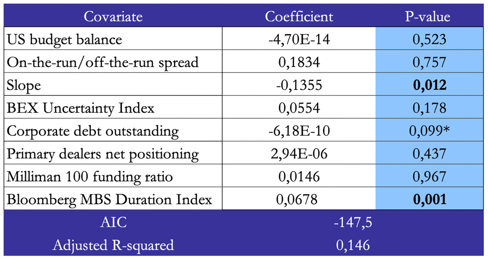
Figure 8: Regression results for LIBOR swap spread in 2008-2012
Source: Bocconi Students Investment Club

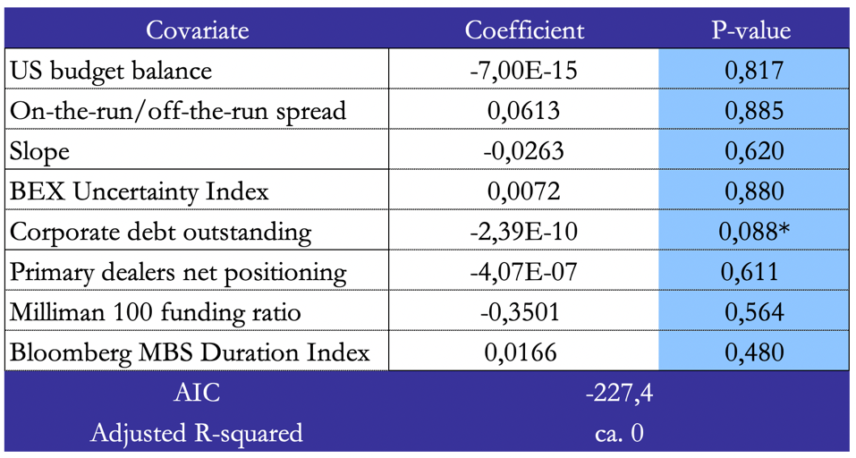
Figure 9: Regression results for LIBOR swap spread in 2013-2017
Source: Bocconi Students Investment Club

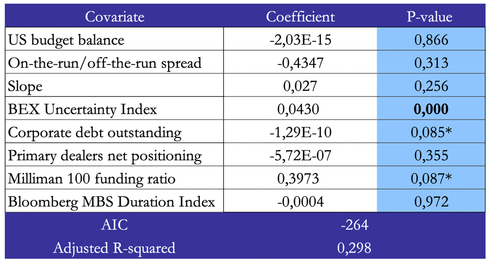
Figure 10: Regression results for LIBOR swap spread in 2018-2022
Source: Bocconi Students Investment Club

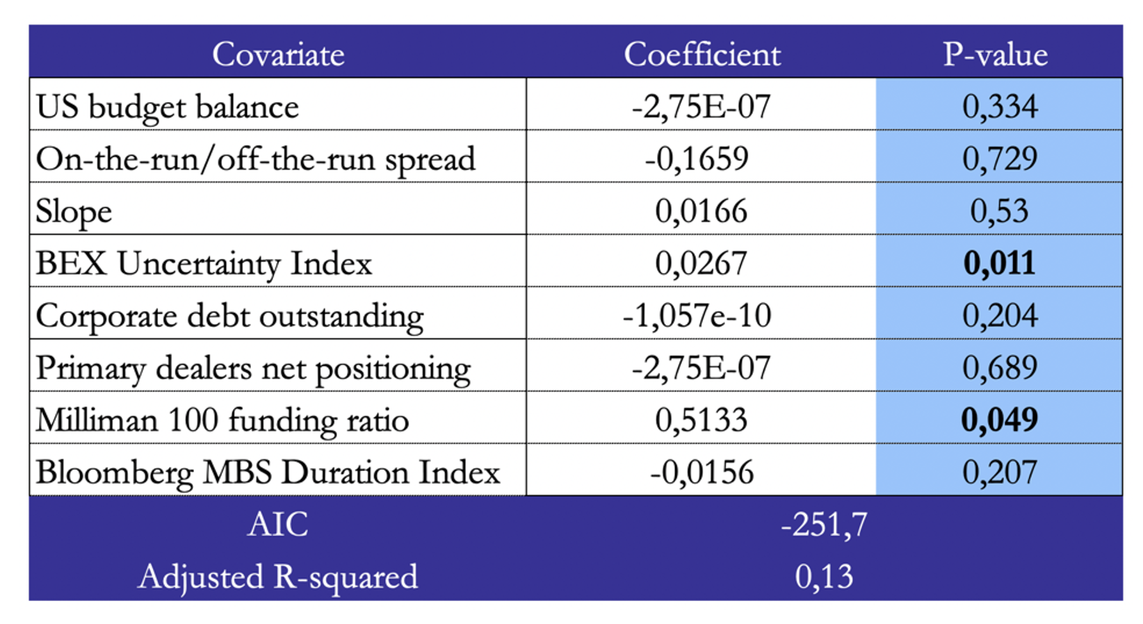
Figure 11: Regression results for SOFR swap spread in 2018-2022
Source: Bocconi Students Investment Club

We find that all regression models have at least one covariate which is statistically significant at a level of 0.95, except for the regression of LIBOR swap spread in 2013-2017. However, we do not identify a statistically significant structural break in the relation between the variables during 2013-2017, despite the introduction of capital regulations in 2015. The significant covariates vary when switching between time periods, with slope of the yield curve and MBS duration becoming insignificant after 2012. During 2018-2022, the BEX Uncertainty Index is a highly significant driver both for LIBOR and SOFR swap spreads, while Milliman 100’s funding ratio is significant only for LIBOR. To conclude, the first model of 2008-2012 is the one that resembles Cortes, 2003 the most, since both MBS Duration and slope of the yield curve are statistically significant and they have the same coefficient signs as Cortes, 2003. After 2012, the drivers change significantly, with our model failing to explain swap spreads during 2013-2017 better than no model. Starting from 2018, uncertainty plays a dominant role both for LIBOR and SOFR swap spreads, together with other demand-based drivers, namely, Milliman 100’s funded ratio and corporate issuance, which are always significant with a p-value lower than 0.10.

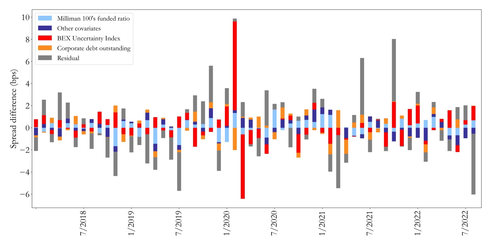
Figure 12: Drivers’ contributions to LIBOR swap spread in 2018-2022
Source: Bocconi Students Investment Club

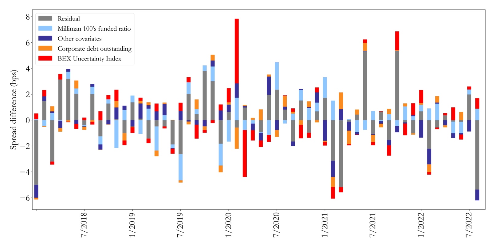
Figure 13: Drivers’ contributions to SOFR swap spread in 2018-2022
Source: Bocconi Students Investment Club

Sources

• Du, Hébert, Li, 2022. “Intermediary Balance Sheets and the Treasury Yield Curve”.
• Hanson, 2022. “Demand-and-Supply Imbalance Risk and Long-Term Swap Spreads”.
• Klinger et al, 2019. “An Explanation of Negative Swap Spreads: Demand for Duration from Underfunded Pension Plans”.
• Boyarchenko et al, 2018. “Negative Swap Spreads”, Federal Reserve Bank of New York.
• Jha, 2011. “Interest Rate Markets”.
• Kobor et al, 2005. “What Determines U.S. Swap Spreads?”, The World Bank.
• Cortes et al, 2003. “Understanding and modelling swap spreads”, Bank of England.

TAGS: swap spreads, swaps, rates, macro, US