Introduction
In 2022, rates traders have had to navigate a landscape of deteriorating liquidity in sovereign debt markets. Over the past few years, there have been multiple episodes of severe illiquidity in US Treasuries and related markets. Firstly, US repo rates spiked in September 2019, with intraday secured overnight funding rates reaching as much as 10% and a day over day increase in interest rates of over 280bps. Secondly, Treasuries experienced decreased liquidity during a selloff in Treasuries in March 2020 which saw 10-year yields increasing by over 60bps in about one week.
In this report, we discuss how to measure Treasury market liquidity, its current state, and the Treasury-Futures Basis trade, which is deeply linked with multiple dynamics that drive liquidity, or its lack.
Measuring Treasury Market Liquidity
As per Fleming (2003), a liquid market is defined by practitioners as “a market with very low transaction costs”. However, since transaction costs depend on a multitude of factors (e.g., the size, timing, venue, and counterparties of a trade) liquidity is not an observable characteristic of a market but has to be inferred through proxies.
According to Fleming (2003), strong liquidity proxies 1. directly quantify transaction costs, 2. behave consistently with the views of market participants, and 3. are easy to calculate and understand. These characteristics are analyzed for the following liquidity proxies: trading volumes, trading frequency, bid-ask spreads, quote sizes, trade sizes, price-impact coefficients, and on-the-run/off-the-run yield spreads.
Most of these measures are easily understood; however, many indicators either do not always behave consistently with the views of market participants, might be hard to attain or do not give a good indication of the real transaction costs. Trading volumes and trading frequency can give misleading signals regarding liquidity since both liquid and illiquid markets are associated with high trading volumes and frequency. The bid-ask spread generally widens in illiquid markets but only indicates the cost of relatively small trades. Quote and trade sizes underestimate the number of securities that could be traded during a day since market makers generally do not quote the total amount of securities they would be willing to trade and real trade sizes are most often lower than the real number of securities that could have been traded at a given price. Price-impact coefficients such as Kyle’s Lambda (see Kyle (1985)) are more computationally intensive than other measures but are generally good indicators of market liquidity. On-the-run/off-the-run spreads are not a direct measure of liquidity but of the liquidity premium and can diverge without meaningful changes in liquidity, but they tend to be accurate.
While none of these measures is flawless, some indicators seem to give a better picture of liquidity than others. In short, price-impact coefficients and the bid-ask spread are historically the best proxies of liquidity. However, real-time price-impact coefficients are harder to obtain than the bid-ask spread and so, keeping in mind the three characteristics of good liquidity measures, the bid-ask spread should be seen as the preferred measure of liquidity in Treasury markets. Together with price-impact coefficients, other modestly strong proxies are quote and trade sizes as well as the on-the-run/off-the-run spread since these generally behave consistently with liquidity observations but not as well as the bid-ask spread. Lastly, trading volumes and frequency can be considered weak proxies of liquidity since a high reading can both indicate high and low phases of liquidity.
The Current State of Treasury Liquidity
Since the end of last 2021/beginning of 2022, Treasury markets have been highly volatile and faced with severe selling pressures due to an increase in inflation, central bank policy rate hikes, and uncertainty around the global economic outlook. Looking at our preferred proxy of liquidity in Treasury markets, the bid-ask spread on 10Y Treasuries, we can observe a noticeable widening since the start of the year, which confirms the decrease in liquidity.

Source: Bloomberg, Bocconi Students Investment Club
Interestingly, this drop in liquidity has been quite orderly and has persisted for much longer than the previously discussed events. This shows that there are more systemic causes of lower liquidity levels rather than an exogenous shock. We find further preliminary evidence for this view in the development of the MOVE Index, which measures implied volatility for 1-month Treasury options and is quite strongly correlated with the above bid-ask spread with a Pearson correlation coefficient of 0.56 (computed over the last 5 years). Since the start of the year, the MOVE Index has been sitting at elevated levels which were lately only topped by the Covid-crash in March 2020, just like the bid-ask spread.
We see two main drivers of low liquidity levels in Treasuries: 1. Significant supply and demand imbalances in the Treasury market and 2. Regulatory burdens on intermediation.
1) Supply and Demand Imbalances
Since the Covid-19 pandemic, supply in Treasury markets has been large to finance fiscal stimulus packages. Simultaneously, the Federal Reserve used its Quantitative Easing (QE) programs to inject unprecedented amounts of liquidity in financial markets. Consequently, supply was high, but it was met by high demand, driven in large parts by the Fed. Now, the Fed has embarked on balance sheet normalization and is no longer buying Treasuries. Additionally, the Treasuries market recorded intense selling pressure as investors priced in inflation and uncertainty risk premia. Meanwhile, supply is still high and net cash raised through Treasuries is on track to reach pre-Covid levels for 2022 as can be seen below.
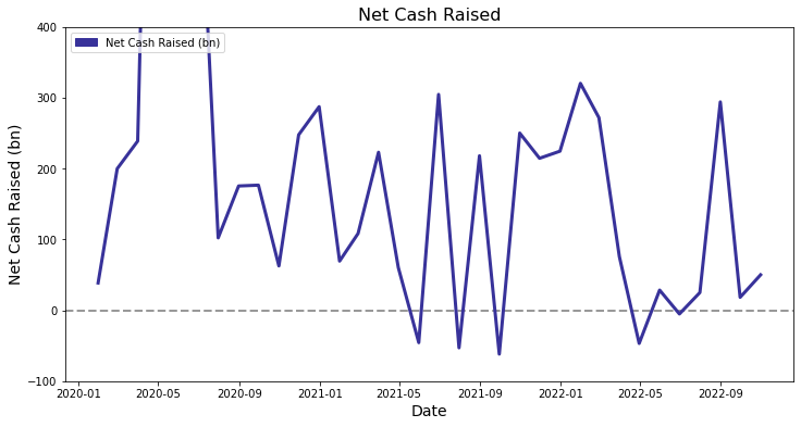
Source: SIFMA, Bocconi Students Investment Club
However, QE and QT are not the only reasons for this imbalance. Firstly, margin calls due to heightened volatility are thought to be another contributing factor to the illiquidity of the Treasury market. Since Treasuries are normally extremely liquid, they are often sold first in the case of a margin call. The fact that interest rates were extremely low for in 2020 and 2021 exacerbated this phenomenon, since market participants increased their leverage leading to even higher margin calls. Two notable examples are 1. the commodities markets and 2. the UK Gilts market, where pension funds were forced to liquidate their government bond holdings to meet margin calls on interest rate swaps. For a more in-depth discussion of the latter topic, we refer the reader to this BSIC Article.
Due to these supply and demand imbalances, there have been calls on the Federal Reserve to start Treasury buybacks. While the Fed has pushed back against buybacks for now, depending on developments in the Treasury market and the economy, there is a possibility for buybacks to take place. Scholars such as Wright (2022) have argued that the current state of the Treasury market and economy could see the Quantitative Tightening process end early. Even just considering buybacks or slowing down QT prematurely speaks volumes about the fragility of the market, not to mention that both measures can lead to moral hazard because market participants know they can rely on the Federal Reserve as a buyer of last resort.
A loosely related (but nevertheless important) factor when looking for the impact of QE and QT on liquidity is discussed at length by Archarya and Rajan (2022) and Archarya et al. (2022). Archarya and Rajan argue that QE enhances the risk of illiquidity for a prolonged period. According to the authors, this might happen because QE increases both the share of assets other than reserves for commercial banks and so-called “claims on liquidity” on the liabilities side (e.g., short-term deposits). These claims on liquidity decrease the “net future availability of liquidity to the [commercial banking] system” since more liabilities are backed up by less reserves. This effect can be especially severe in times of crisis, where demand for reserves may exceed their supply. Archarya et al. (2022) add to this by showing that banks substantially increase claims on liquidity during periods of QE but do not subsequently reduce these claims during periods of QT and therefore become more prone to liquidity stress. These problems could then spill over into other markets such as Treasuries if banks are forced to liquidate parts of their assets to serve demand of customers.
2) Regulatory Factors
Since the Great Financial Crisis (GFC) of 2007/08, regulation has increased capital requirements of banks and has focused more on the role of intermediaries in financial markets. The most famous examples of these reforms are the Dodd-Frank Act and the Basel II & III accords. The figure below shows bank capital as a percentage of total public debt. We see that while bank capital (defined as total assets less total liabilities of banks) has increased, it has not kept up with total debt outstanding (i.e. a proxy for the size of the Treasury market). And since we can use bank capital as a proxy for the intermediation capacity of banks, this chart shows that this intermediation capacity has gone down significantly over the past 15 years.
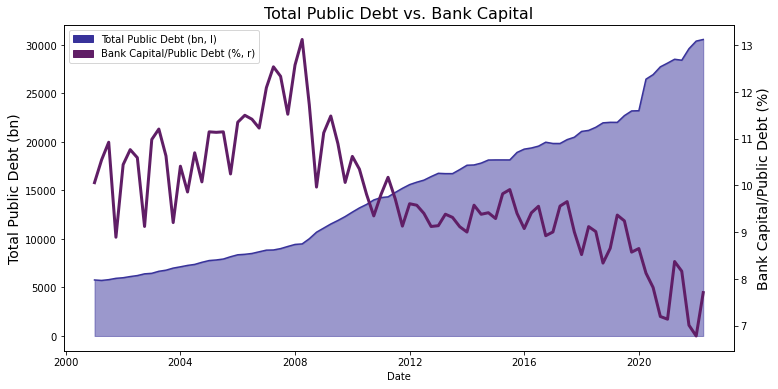
Source: FRED, Bocconi Students Investment Club
Turning to total Treasuries outstanding, we see that banking institutions not only hold a higher absolute level of Treasuries but also hold more of the Treasury market as a whole on their balance sheets as evidenced by the graph below. A possible explanation are high quality liquid asset constraints.
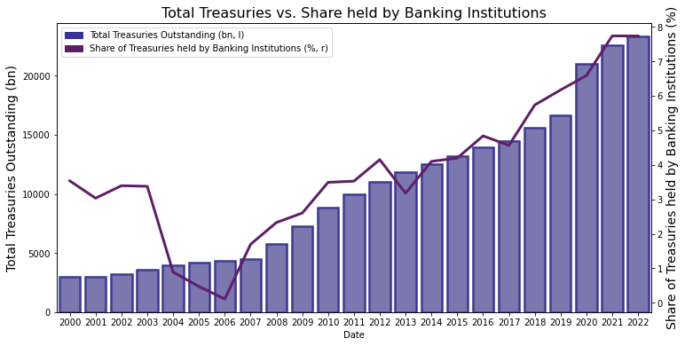
Source: SIFMA, Bocconi Students Investment Club
At the same time, reserve requirements and leverage regulations such as the supplementary leverage ratio force banks to hold reserves for their Treasury holdings. This has made it more expensive for banks to intermediate in the Treasury markets, and intermediation has shifted to a technology-heavy and asset-light approach. As a consequence, average primary dealer transaction volume relative to total Treasury outstanding has plummeted from about 14% to under 3%.
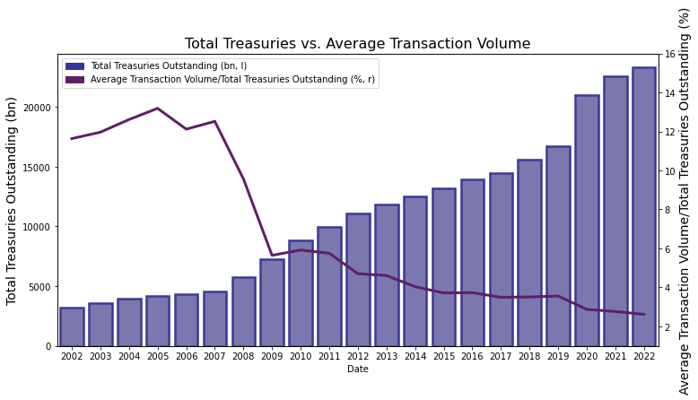
Source: SIFMA, Bocconi Students Investment Club
To sum up, the drivers for the current illiquidity in Treasury markets and the frequency of liquidity stress differ. While the former is driven both by regulation as well as by intense selling pressure without adequate demand, the latter is mainly driven by regulation. Therefore, we believe that Treasury markets will become more liquid once the economic outlook clears up, but liquidity shocks might become more frequent.
Basis trading
Having discussed illiquidity and its main drivers, we now introduce the bond-futures basis trade, a trading strategy that caused large losses for multiple hedge funds in March 2020 when Treasury liquidity deteriorated. The gradual retreat of the Federal Reserve from Treasury markets via QT has led to a comeback of basis trading in 2022, but the ongoing liquidity crisis in US interest rate markets might pose some threats (and present opportunities) in the Relative Value (RV) space. Before discussing basis trading, we introduce the main features of bond futures contracts.
Bond Futures contracts are different from other financial futures in that they are not written on a specific underlying asset, but on a notional bond (generally) with a 6% coupon. To illustrate the contract specifications for Treasury Futures contracts, we reproduce below a table by the CME Group:
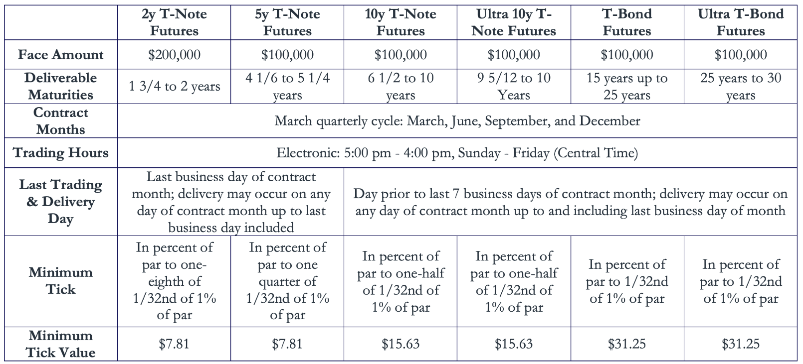
Source: CME Group
The deliverable issue in a bond futures contract is not a specific bond, but one in a basket defined as in the table above. This is done to limit the risk of failure-to-deliver by the short party in the futures contract, who needs to source the bond. The existence of a delivery basket requires a system to make the long and short parties indifferent as to which issue will be delivered. To each issue in the delivery basket is associated a conversion factor (CF), which adjusts the price of the bond so that its YTM at futures delivery equals the coupon of the notional bond.
The CF is fixed for each issue in the delivery basket when the futures contract starts trading. The CF system is however far from perfect: it assumes a flat term structure and that all bonds trade at the same yield. As a result of changing prices in the delivery basket, one bond is cheapest to deliver (CTD). The CTD is the bond that gives the greatest return from the cash and carry strategy of buying a bond and selling the futures contract, and then closing out positions on expiry of the contract. The next figure explains two ways to identify the CTD.
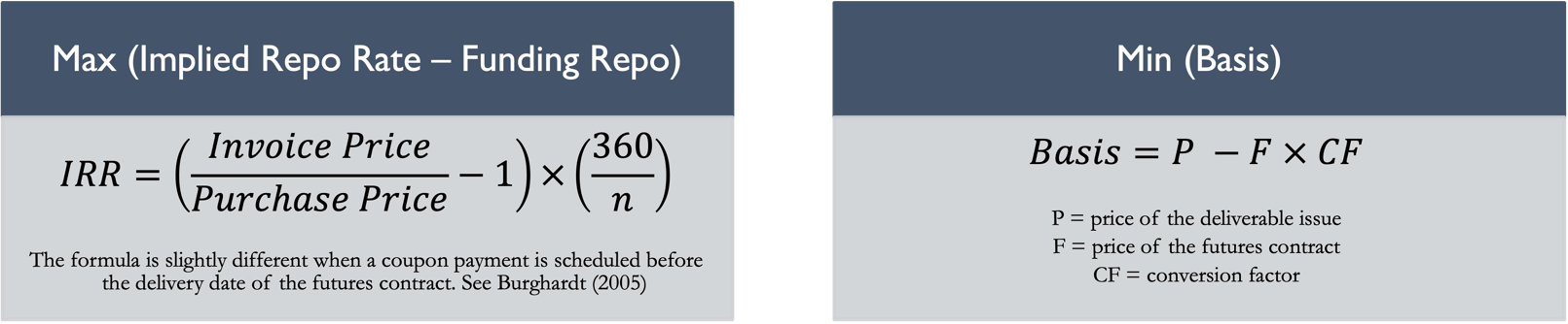
Source: Bocconi Students Investment Club
The implied repo rate is the rate of return from a cash and carry strategy implied by the current prices of the futures contract and the deliverable issue. The basis is the spread between the price of the deliverable issue and the converted price of the futures contract. When the basis is adjusted for carry, it is referred to as net basis (BNOC).
The basis between bonds and their futures, and especially the Treasury-Futures basis, is more complex than bases in other financial or non-financial futures contracts and other types of spot-derivative bases because of its embedded optionalities. The delivery basket system and the existence of a CTD give rise to a quality option for the short party, who can decide which issue to deliver at expiry of the futures contract. For US Treasury Futures (CBOT), timing options are also granted to the short position, while for EGB Futures (Eurex) they are negligible. The short party can choose when to make delivery within the contract month, giving rise to a carry option. Delivery can be made after the futures contract stops trading, i.e., 7 business day before the end of the month. During that time interval, the futures price is fixed, while the spot price of the issues in the delivery basket can change. This difference defines the payoff of the end-of-month option. Finally, in the period from 2:00 p.m. to 7:00 p.m. (Chicago time) every day when the futures market is closed but bonds keep trading, if there is enough volatility, there can be a change in the IRR, changing the payoff of the basis position. The option to make delivery after 2:00 p.m. is called wildcard option.
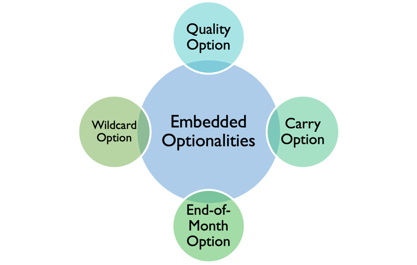
Source: Bocconi Students Investment Club
Having introduced the functioning of bond futures contracts, we now present the mechanics and dynamics of basis trading (focusing on US Treasuries), one of the most popular fixed income RV strategies. Basis trading spans three key interest rate markets: the US Treasury market, the Treasury Futures markets, and the Repo market. Because of its three-legged nature, all the topics we discuss in this report play a role in determining returns in basis trading. In the diagrams below we explain the structure of a long basis trade. The choice of going long the basis is for illustration purposes only. The short basis trade is conceptually analogous, with the CTD being sold short through a reverse repo where the hedge fund lends cash in a transaction collateralized by the CTD and then sells the issue in the cash market.
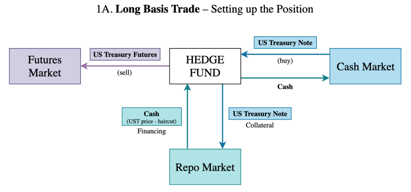
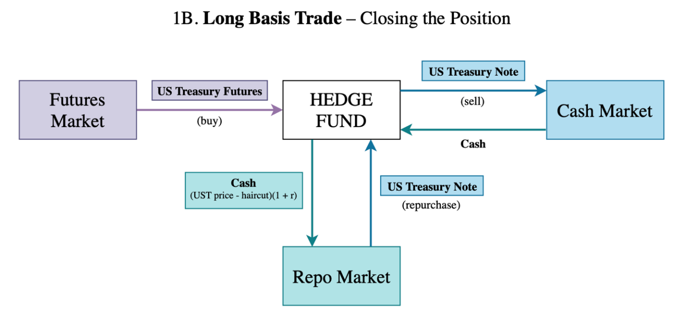
Source: Bocconi Students Investment Club
1) Basis trading and optionality
It is important to understand that a long basis trade is not an arbitrage. As we discussed above, the BNOC represents pure optionality, indicating that it should stay positive until the futures expires. A negative BNOC, on the other hand, does represent an arbitrage opportunity, insomuch as it amounts to free optionality, but it is not entirely uncommon, for instance due to capital constraints in times of crises. Therefore, a long basis position is better understood as a form of yield enhancement rather than arbitrage. If the CTD doesn’t change, the basis converges to 0 when the contract (and the embedded options) expires. However, the CTD can change, leading to basis widening. In that case, the return from the long basis position would exceed the IRR.
The IRR is generally marginally lower than returns on bills (if we do not account for leverage due to repo financing), despite having a similar risk profile (assuming low repo rollover risk and small margin requirements, which can be financed at an unsecured rate), see Barth and Kahn (2020). This is again due to the embedded optionalities. In other words, the short party needs to pay for the rights she is granted by her long basis position.
Two things are clear then: a long basis position is a long option position, and being long the basis, just like being long an option, amounts to being long volatility. What has not emerged yet is whether the long basis position is akin to a call or put option, but that is a function of where market yields stand with respect to the 6% coupon of the notional underlying bond. If yields are below 6%, which has been the case for the past two decades, the deliverable issue with shortest duration tends to be CTD. Then, if rates rise, the CTD is likely to change (because bonds with longer durations will drop more in price) and the basis to advance (the CTD minimizes the basis), and vice versa if rates fall. Thus, going long the basis is equivalent to buying a put option, which has limited downside (the basis can go to 0) and theoretically unlimited upside. On the other hand, if yields are above 6%, a long basis position is akin to a call option since the longest duration issue is generally the CTD. Yields in a neighborhood of 6% would lead the basis to resemble a straddle. Notice, however, that the above reasoning is correct if we limit our analysis to parallel shifts in the term structure of interest rates.
2) Basis trading, liquidity, and scarcity
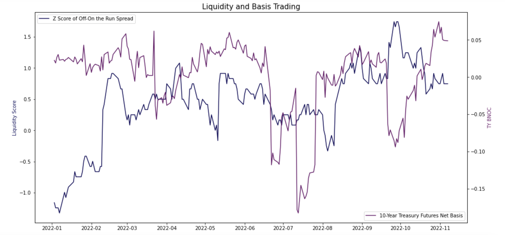
Other important considerations in basis trading are liquidity and the availability of the CTD. The basis is expected to advance when the deliverable issue trades on special, because the cost of carry is lower. Thus, high demand and limited availability of the CTD drive the basis. As explained by Duffie (1996), the most liquid issues tend to trade on special in the repo market. Since the CTD tends to be a highly liquid issue in EGBs, as shown by Ejsing and Sihvonen (2009), it is not unusual for it to trade on special, especially during flight-to-quality or flight-to-liquidity episodes. In the US, however, liquidity premia are priced in on-the-runs more than in CTDs. Hence, we expect flight-to-liquidity episodes to have a much more limited impact on the basis, if any. In fact, as we show in the figure below, the BNOC for 10-Year Treasury Futures (TY) has often been negative in 2022, while the liquidity premium (measured by the spread between first off-the-run and on-the-run YTM) has been quite large. The two series have a negative correlation coefficient of -16%, indicating that preference for liquidity in US rates markets doesn’t seem to support the Treasury-Futures basis.
Source: Bloomberg, Bocconi Students Investment Club
3) Basis trading and regulations
As we have highlighted earlier in this report, regulatory changes after the crisis of subprime lending and the subsequent GFC have contributed to higher costs of liquidity provision by dealers and constrained intermediation capacity. It turns out, as clearly evidenced by Fleckenstein and Longstaff (2020) and Boyarchenko et al. (2022) that regulatory changes have also made “arbitrage”-style activities, such as trading the basis, more expensive for banks and security dealers and, indirectly, also for hedge funds.
As Fleckenstein and Longstaff (2020) points out, derivatives intermediation is often more expensive for dealers because they also need to trade the underlying to hedge the risk on their book. They build a simple model where dealers hedge themselves fully and face simple costs including repo financing for the long position in the Treasury Note and unsecured funding for futures margin, the repo haircut, and other costs.
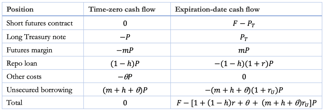
Source: Fleckenstein and Longstaff (2020)
Their simple model illustrates how an investor opening a long position in a Treasury Futures contract is in fact renting balance sheet space and paying for it. In this setting, the spread between the IRR on the futures and the carry costs on the US Treasury Note represents the cost incurred by the investor for renting space on the dealer’s balance sheet. The usefulness of this model is also numerical: the authors use the formula to estimate the component of the basis that is related to intermediation costs. Their results “provide direct evidence that the funding basis is driven by changes in balance sheet usage costs”.
Similar conclusions are reached by Boyarchenko et al. (2022), who look at the difference between basis trading costs under risk-weighted-asset (RWA) regulations and post-GFC supplementary leverage ratio (SLR) regulations. Under RWA requirements, repo positions to finance the long Treasury position of the basis trade do not affect the leverage ratio, as they do not impact the Tier 1 capital in the numerator of the ratio. Under SLR requirements, however, the full notional of repo transactions is recognized as leverage, even if the repo is collateralized by US Treasuries, the safest assets in the world. Hence, the SLR “requires significantly more capital against relatively low-risk, low-margin activities such as repo borrowing and lending against Treasury securities” (see Boyarchenko et al. (2022)). On balance, the required return on the basis trade that would make it worth to bear these burdensome leverage costs for the dealer are too high, effectively discouraging them from engaging in basis trading. The authors find that these regulatory changes have led to wider spot-derivative bases on average in post-GFC times.
Sources
[1] Fleming, 2003. “Measuring Treasury Market Liquidity”.
[2] Kyle, 1985, “Continuous Auctions and Insider Trading”.
[3] Board of Governors of the Federal Reserve System, 2022. “Financial Stability Report, November 2022”.
[4] Wright, 2022. “Shrinking the Fed Balance Sheet”.
[5] Acharya, V. and Rajan, R. 2022. “Liquidity, Liquidity everywhere, not a Drop to Use – Why flooding Banks with Central Bank Reserves may not expand Liquidity”.
[6] Acharya et al. 2022. “Liquidity Dependence: Why Shrinking Central Bank Balance Sheets is an Uphill Task”.
[7] Scheicher, M and Schrimpf, A. 2022. “Liquidity in bond markets – navigating in troubled waters”.
[8] Boyarchenko et al., 2022. “Bank-Intermediated Arbitrage”. FRB of New York Staff Report No. 858.
[9] Barth, D. & Kahn, J., 2020. “Basis Trades and Treasury Market Illiquidity”. Briefs 20-01, Office of Financial Research, US Department of the Treasury.
[10] Duffie, D., 1996. “Special Repo Rates”. The Journal of Finance, 51: 493-526.
[11] Ejsing, J. & Sihvonen, J., 2009. “Liquidity premia in German government bonds”. Working Paper Series 1081, European Central Bank.
[12] Fleckenstein, M. and Longstaff, F. A., 2020. “Renting Balance Sheet Space: Intermediary Balance Sheet Rental Costs and the Valuation of Derivatives”. The Review of Financial Studies, Volume 33, Issue 11, Pages 5051–5091.
[13] Burghardt, G., and T. M. Belton. 2005. “The Treasury bond basis–An in-depth analysis for hedgers”, 3rd ed. New York: McGraw-Hill Professional.


0 Comments