Modeling Asset Correlation: Theory and Practice

Download PDF

Introduction

Correlation is a pervasive concept in financial markets. It is studied by investors looking for the most reliable way to hedge their exposure while financial products that offer a directional correlation exposure also became substantially more liquid in recent years. Moreover, the substantial mispricing of correlation risk in mortgage-backed securities (MBS) is seen as key trigger of the subprime crisis. In last week’s article, we discussed this year’s correlation breakdown, presented ways to trade correlation and pitched a trade based on the current macroenvironment. In this article, we focus on correlation modeling that is key for asset pricing and risk management. It is structured as follows. In the first part, we introduce commonly employed econometric correlation models and discuss their merits. The second part presents applications of these correlation models for several asset classes.

Primer on Covariance and Correlation Modeling

When modeling correlation, researchers commonly face two main empirical challenges. First, when univariate models are extended to the multivariate case to include asset correlations, the number of degrees of freedom rapidly declines. The addition of one asset in a variance-covariance model of a portfolio consisting of assets requires not only the estimation of the asset’s own variance but also of covariances. For large portfolios, as commonly employed in asset and risk management, this could substantially undermine the parameters’ stability. Second, estimation parameters must often be restricted to lead to positive portfolio variances, further complicating the procedure. Also, the correlation between two assets must be bounded to ensure the interpretability as correlation coefficient, i.e. .

Like models of the return variance, the estimation and forecasting of covariances and correlations concerns the second moment of financial variables. Variance models therefore constitute a natural starting point for extensions to correlation modeling. A brief introduction to these models can be found here. Due to its importance and similarity with more advanced models presented later on, we only repeat the baseline GARCH(1,1) model at this point, which can be defined as follows:

Here, the forecasted variance is dependent on last period’s squared prediction error of returns and the preceding variance forecast . The term ω is an intercept and the long-run variance can be expressed by . This model is not only parsimonious but was also commonly shown to outperform more complex models.

The most direct extension of the GARCH(1,1) model is the so-called VECH-GARCH(1,1) model which for the case of two assets can be written as:

In this model, all assets’ variances and their respective covariances are dependent on the errors from a mean model and the previous variance forecasts ( for covariance). The model is called vectorized, as duplicate elements from the symmetric variance-covariance matrix are dropped in this form. While the model retains the parsimony of the univariate case, as described above, it suffers from the low number of degrees of freedom for many assets. For assets, it requires the estimation of parameters. Two methods can be employed to mitigate this issue. First, the intercept term can be restricted to ensure that the model’s long-run variances and covariances match their sample counterparts. Second, a diagonal structure can be imposed on the matrices A and B. This is equivalent to assuming that there exists no direct interdependence between variances and covariances but both processes are driven by the errors from the conditional mean model.

A final limitation of this model concerns the fact that the estimation does not ensure a strictly positive variance of any portfolio consisting of the N assets, requiring further restrictions on the parameters. The Baba-Engle-Kraft-Kroner (BEKK) GARCH(1,1) model offers an improvement in this regard. It can be expressed in matrix form as follows:

This model preserves the structure of the initial GARCH model with the main extension being the quadratic structure of the coefficient matrices and . While this appears to be a technical detail, it simplifies the estimation substantially as it automatically ensures that all portfolios consisting of the N assets in the model have positive variances without imposing further parameter restrictions. A further advantage of the model is its linearity feature. This represents the fact that if all assets individually follow a BEKK GARCH process, all portfolios formed from them can also be modeled by the same process. While the model therefore mitigates some of the VECH GARCH’s drawbacks, it still requires the estimation of a large number of parameters (although the number is growing by the factor of instead of as before). To increase the degrees of freedom, researchers therefore commonly impose a diagonal structure on A and B with similar implications as described for the VECH GARCH model.

Finally, the dynamic conditional correlation (DCC) model takes a slightly different approach to the previously presented models by directly modeling correlation instead of estimating covariances beforehand. Its estimation follows a two-step procedure. First, all assets’ variances are independently modeled, e.g. by employing a univariate GARCH model. In the second step, the residuals of these models are standardized by the respective standard deviations. These values are then used to estimate the time-varying correlation by:

Thereby, denotes the standardized errors from the first-stage model and is the long-run correlation which is usually set to equal the sample correlation between the two respective assets. Note that the dependent variable is an auxiliary variable that can be translated into the correlation forecast by .

This model possesses two key advantages. First, the use of the auxiliary variable ensures that the obtained correlation forecast is always in the range of [-1,1] while also satisfying the condition of a positive variance for all combination of assets. Second, the two-step approach of the DCC allows researchers to estimate correlation matrices even for large portfolios, as the number of estimated parameters only depends on the structure of the second stage model and is therefore independent of the number of assets under consideration. Besides these improvements to the models presented above, the DCC preserves a high degree of flexibility. By restricting covariance targeting can be implemented, while also the inclusion of asymmetric effects is possible. The latter point could be relevant when simultaneous upward surprises in the variances of both variables are assumed to have a different impact on correlation than shocks with different signs. This seems especially relevant due to the observation that asset correlations commonly increase substantially in bear markets (and therefore supposedly when variances spike).

Aielli (2013) discusses some of the issues present when using the Dynamic Conditional Correlation (DCC) model and proposes a more refined model called cDCC (corrected DCC). This improved model solves the lack of consistency of the DCC model and the hardships in the traditional GARCH-like interpretation of dynamic correlation parameters. The author proves the heuristic consistency of a large system estimator for the cDCC model and derives sufficient conditions for the stationarity requirements. The associated cDCC estimator produced results that were essentially consistently unbiased. Besides, the cDCC correlation forecasts performed similarly to or better than the DCC correlation forecasts in applications to real data.

The main contribution of Aielli (2013) is to draw attention to the issue of inconsistency, but the suggested solution still has the same issues as the DCC representation. In fact, Aielli (2013) talks about targeting and a change to DCC that makes consistent estimates possible. But he makes the unstated assumption that the estimators of the modified DCC representation are asymptotically normal under standard regularity requirements. Caporin and McAleer (2012) demonstrated that while asymptotic normality cannot be proved, dynamic conditional correlations may be reliably predicted using an indirect DCC representation based on the BEKK model.

Applications of DCCs

Next, we will look at how the DCC model has been applied in the financial literature and focus on papers analyzing financial contagion. They usually offer a good perspective on how spillovers occur and their main drivers.

Syllignakis and Kouretas (2011) examines the time-varying conditional correlations to the weekly index returns of seven emerging stock markets in Central and Eastern Europe using the DCC model. To capture possible ripple effects across the US, German, Russian, and Central and Eastern Europe (CEE) stock markets, they analyzed weekly data from 1997 through 2009. They discovered evidence of increased conditional correlation spread between the USA, Germany, and the CEE stock markets during the GFC and supposed that the exchange rate movement could explain the crisis from 2007–2008. Celık (2012) also employed the DCC model and presented evidence of US contagion to the most developed and developing economies, finding out that the latter were most impacted by the US subprime crisis.

According to Akhtaruzzaman et al. (2021), financial contagion between China and the G7 nations during the COVID-19 period could happen through both financial and non-financial enterprises. The empirical findings demonstrate that listed companies in these nations, including financial and non-financial corporations, see a notable rise in conditional correlations between their stock performances. Nonetheless, during the COVID-19 epidemic, the magnitude of the increase in these correlations is much higher for financial businesses, highlighting the significance of their participation in the spread of financial contagion. Additionally, they demonstrate that, in most situations, ideal hedge ratios rise noticeably, indicating an increase in hedging expenses for the COVID-19 period.

Application I: Modeling FX Correlations

In the following section, we display a simple application of DCC models in FX markets. For this, we employ a dataset of weekly observations starting from November 2002 to analyze the dynamic correlation behavior of G10 currencies. Note that, where necessary, we have inverted the usual notation of exchange rates to consistently have USD as quote currency. This is industry standard and enhances comprehensibility as a positive correlation between two currencies with respect to the USD thereby implies a simultaneous strengthening or weakening of the non-USD currencies.

The use of the DCC model enables us to estimate time-varying correlation matrices for our case of assets without suffering from a dimensionality problem. We employ a simple GARCH(1,1)-DCC model as described above. The estimation yields highly significant parameters and indicates an overall persistence around 0.94.

For reasons of conciseness, we only present a short excerpt from the estimation. The chart below shows the estimated dynamic conditional correlations of the Norwegian Krone with the Australian Dollar and the Japanese Yen, respectively. Several features of this result appear striking. First, although both countries have an equally low degree of integration with Norway’s economy, there exists a substantial gap in the correlation levels. Further, while the NOK-AUD correlation is rather stable at a high level, the NOK-JPY correlation is more volatile over time. These observations can largely be explained by the “beta” of these currencies. Both NOK and AUD are known as “high-beta” currencies due to their respective economies’ strong reliance on commodity exports. This leads to a high correlation of the currencies with commodity prices and risk sentiment. JPY on the other hand, was especially in the early 2000s commonly seen as a “safe haven” performing well in times of turmoil. See here for a more recent evaluation of this property. This explains the substantial decrease in correlation around 2008, even turning negative with JPY strengthening against USD.

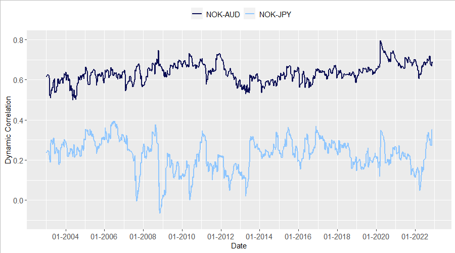
Source: Bloomberg, Bocconi Students Investment Club

Application II: Modeling Equity Contagion

Source: Bloomberg, Bocconi Students Investment Club

Next, we will look at another application of the DCC model, namely correlation modeling in the case of stock returns (S&P 500, DAX, FTSE 100, Nikkei 225). We use the weekly logarithmic returns from January 2019 until November 2022 for the four stock indices and implement a GARCH (1,1)-DCC model to obtain the dynamic conditional correlation time series. The stability condition is met, and both coefficients are highly significant.

Market return correlations often go down during bull markets and rise during downturn ones. Additionally, it is widely accepted that there is a considerable increase in international stock market correlation during periods of market volatility (i.e., stock market crises). From the figure above, we can observe that during the COVID-19 period, correlation significantly increased in February-March 2020 and had a mainly descending trend thereafter, when the volatility calmed down. The Japanese index is less correlated with the other indices, even if it may exhibit spikes in periods of high uncertainty. Only the correlation with the UK index is shown in the figure but similar results hold for the other ones. On the other hand, it is curious to observe that the correlations between European and global economies went down dramatically when Russia invaded Ukraine, showing the partially isolated characteristic of the market shock.

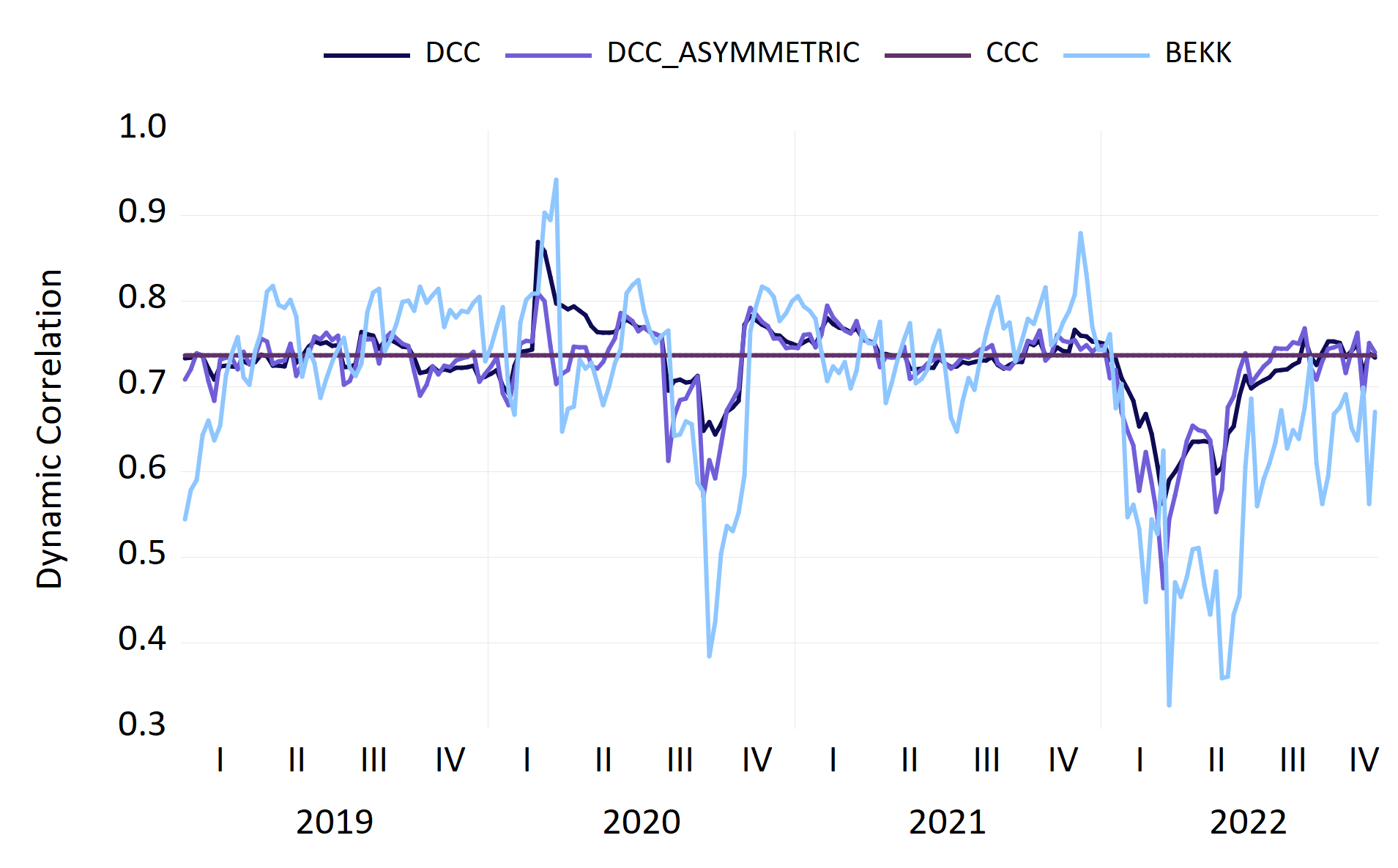
Source: Bloomberg, Bocconi Students Investment Club

In this figure, we observe the behavior of different correlation models for German and American stock market returns (using the same dataset as above). The CCC model is not very insightful in understanding the dynamics of correlations over time, as it estimates a constant correlation for the entire analyzed period. Also, the diagonal BEKK-GARCH (1,1) model is more volatile than the DCC and asymmetric DCC models. The latter type of DCC includes asymmetries, which occur when the impact of two positive shocks differs from the impact of two negative shocks of the same magnitude or the impact of two shocks with opposite signs.

Conclusion

In this article, we presented an introduction to the main models for asset correlation and displayed several use cases in the academic literature. Additionally, we presented two applications for FX, as well as equity markets and compared the performance of different statistical models.

Sources

[1] Aielli, G. P. (2013), “Dynamic Conditional Correlation: On Properties and Estimation”, Journal of Business & Economic Statistics

[2] Caporin, M. and McAleer, M. (2012), “Do We Really Need Both BEKK and DCC? A Tale of Two Multivariate GARCH Models”, Journal of Economic Surveys

[3] Caporin, M., and McAleer, M. (2013), “Ten Things You Should Know about the Dynamic Conditional Correlation Representation”, Econometrics

[4] Guidolin, Massimo, and Manuela Pedio (2018), “Essentials of time series for financial applications”, Academic Press.

[5] Syllignakis, M.N. and Kouretas, G.P. (2011), “Dynamic correlation analysis of financial contagion: evidence from the Central and Eastern European markets”, International Review of Economics & Finance

[6] Celık, S. (2012), “The more contagion effect on emerging markets: the evidence of DCC-GARCH model”, Economic Modelling

[7] Akhtaruzzaman M, Boubaker S, Sensoy A (2021), “Financial contagion during COVID-19 crisis”, Financ Res Lett.