“Well, CAN THEY PREDICT?”: An investigation of Crypto Prediction Contracts’

Introduction

Prediction markets have long been touted as effective aggregators of information, leveraging the collective intelligence of participants to generate probability estimates for real-world events. Platforms like Kalshi have taken this concept a step further by allowing users to speculate on a broad range of outcomes, from political events to macroeconomic trends. Among the most actively traded contracts are those tied to the future price of Bitcoin, where participants can bet on whether the cryptocurrency will surpass a specified threshold by a given date. These contracts resemble European digital options, with their payouts contingent on the occurrence of a binary event at expiration.

In the absence of institutional traders and with relatively low liquidity, markets like Kalshi may exhibit inefficiencies that lead to systematic mispricings. Our objective in this analysis is to test whether such discrepancies exist through various stochastic approaches as well as a direct comparison of probabilities vis-a-vis cryptocurrency exchange options such as Deribit. By comparing our estimated probabilities to those observed in Kalshi’s contracts, we aim to assess whether traders in these decentralized markets systematically misprice Bitcoin’s likelihood of reaching specific price levels.

This analysis carries implications beyond cryptocurrency speculation. If inefficiencies persist due to structural limitations—such as liquidity constraints, behavioural biases, or a lack of institutional arbitrageurs—then prediction markets may not always price probabilities correctly. In turn, this could open opportunities for informed traders to exploit mispricings, while also raising questions about the broader accuracy of decentralized forecasting mechanisms. By applying a rigorous quantitative framework, we seek to bridge the gap between theoretical pricing models and real-world prediction market behaviour, ultimately shedding light on the efficiency of markets where financial derivatives and betting mechanisms converge.

Cryptocurrency Contracts

On Kalshi, the contracts offered are presented as binary prediction markets—simply called “markets”—where each market poses a yes/no question about a real-world event. When it comes to forecasting the prices of cryptocurrencies like Bitcoin, Ethereum, or XRP, the markets are typically framed with questions such as “Will Bitcoin be above $100,000 on [date]?” or “Will Ethereum reach $3,000 by [date]?” These markets are structured so that each outcome is represented by a share that trades between $0.00 and $1.00 USDC, reflecting the market’s perceived probability of the event occurring.

Even though Kalshi does not explicitly label these instruments as “European Digital” or “American One Touch” options, their payoff profiles are strikingly similar to those familiar in traditional finance. A market based on a fixed threshold—like the one asking if Bitcoin will exceed a specific price at market close—behaves much like a European Digital (or Double Digital) option, delivering an all-or-nothing payout at expiration. In contrast, a market that triggers a payout immediately upon the asset hitting a certain barrier during the contract’s lifespan mirrors the structure of an American One Touch (OT) option. For the purpose of this article, we will focus on contracts that behave like European Digital options.

A graph showing a line AI-generated content may be incorrect.

Contract Pricing

The question that this article wants to answer is: how do we decide if one of these contracts is correctly priced? To this end we will focus on the pricing of European digital contracts on Bitcoin.

No-arbitrage pricing suggests that the price of any contingent claim is equal to the discounted value of its risk-neutral expected payoff. In the following section we will explore how we can obtain the risk-neutral distribution from which this price can be derived. In particular we will focus on three approaches in this article.

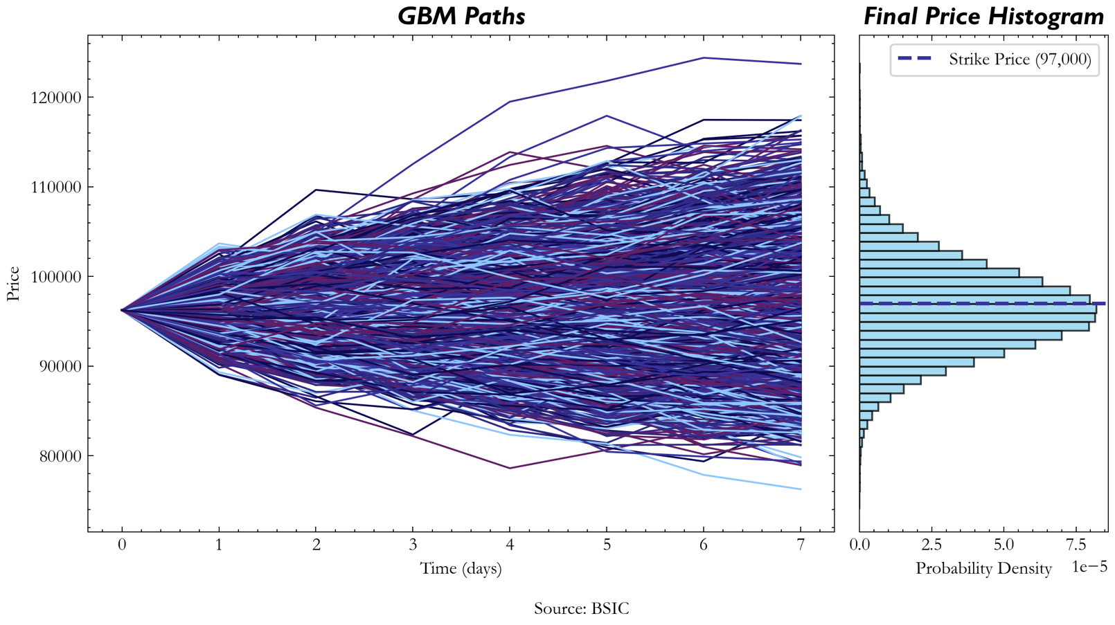
The first approach to evaluating potential market inefficiencies on platforms like Kalshi involves using a Monte Carlo simulation based on a jump-diffusion model. This model extends the classic geometric Brownian motion by incorporating both continuous price movements and discrete jumps, thereby capturing the complex dynamics observed in assets such as Bitcoin. By simulating a range of possible price paths and comparing the resulting distribution to an expected, theoretically efficient market distribution, we aim to identify systematic deviations that could indicate mispricings and underlying market inefficiencies. The underlying formula for this process is the following:

$S_t = S_0 \cdot \exp\left( \left(\mu - \frac{\sigma^2}{2}\right)t + \sigma W_t \right)$

Where, $\mu$ denotes the drift rate or expected return, $\sigma$ represents the volatility of the asset, and $W_t$ is standard Brownian motion, capturing the random movements in the market. A correction factor derived from Itô’s lemma is also applied, adjusting for the impact of the randomness introduced by volatility.

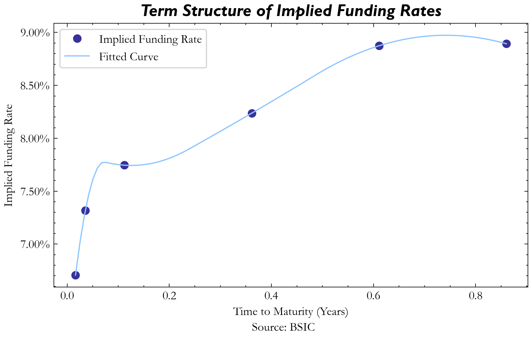
In financial literature, $\mu$ is typically set as the risk-free-rate to ensure no-arbitrage constraints are, generally, respected within GBM simulations. A common proxy for such a rate would naturally be something along the lines of the 3-month US T-Bill annualized yield. However, in the case of Bitcoin, our findings across various cryptocurrency exchanges suggested that the basis observed between Bitcoin’s spot and futures contract implied funding rates in excess of the risk-free rate. A potential explanation of this discrepancy could be found in the fact that BTC returns tend to be quite volatile relative to other financial assets. Furthermore, arbitraging such an opportunity via cash-and-carry with leverage would likely require a substantial amount of initial margin to be posted in order to absorb volatile shocks in price action. Considering this fact, our models’ $mu$ term reflects the basis for the expiry we want to analyze. We report here the term structure of the implied funding rates priced in BTC futures.

A graph with a line and dots AI-generated content may be incorrect.

Next, we recognized that utilizing a standard GBM model with a constant volatility term could be problematic when trying to model BTC price action. This is because of the nature of the GBM model: it tends to underestimate outlier events due to the thinner-tailed nature of lognormal distributions. Hence, in order to introduce the volatility needed for fatter tails on a standard GBM model, a stochastic volatility term was decided upon. The volatility term itself was calculated using Riskmetrics:

$\sigma_{t}^2 = \lambda \,\sigma_{t-1}^2 + (1 - \lambda)\, r_{t-1}^2$

Where $\sigma_{t}^2$ represents the estimated variance at time $t$ , $\r_{t-1}^2$ and $\lambda$ is a decay parameter, which empirically performs optimally around 0.94. The intuition behind the Riskmetrics lies within the decay term; as time $t$ approaches the end of the simulation, lambda exponentially decreases the weighting of previous variance terms and places increased emphasis on previous squared log returns. This follows the logic that recent volatility should bear higher meaning as opposed to far-removed volatility observations from old time series data.

So, how is Riskmetrics being implemented within the GBM? Firstly, in order to gain an initial volatility estimate to kickstart our GBM, we used Riskmetrics to provide an EWMA of previous variances and took the most recent daily volatility estimate. However, that wasn’t its only purpose: it was also used at each step across every path in our simulation, using the previous log return of that respective path to inform its next value. This way, there’s an increased degree of variability in our final distribution, leading us to those desired fat-tails.

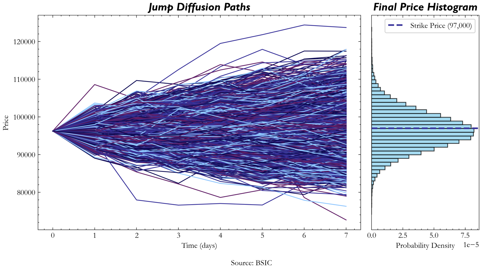
As an alternative to GBM with stochastic volatility, the standard GBM model can be further refined by incorporating jump diffusion. This approach enhances the model’s realism by adding a component that accounts for sudden, discrete price movements—events that are not adequately captured by the continuous nature of GBM. The formula for a standard Jump diffusion model is given by:

$[ dS_t = \mu S_t , dt + \sigma S_t , dW_t + S_t , dJ_t, ]$

Here, the only difference between this model and a standard GBM is the $dJt$ term which represents the jump component. This component is expressed the following way

$[ dJ_t = \left(e^Y - 1\right) dN_t, ]$

In which $N_T$ is a Poisson process which accounts for the number of jumps up to time $t$ , where $dN_t$ can either take the value of 1 (a jump occurs) or 0 (a jump doesn’t occur). The probability of a jump is represented by the intensity term $\lambda$ multiplied by the time increment $d_t$ . When $dN_t$ takes the value of 1 (the jump occurs), its size is represented by the $e^Y - 1$ term where $Y$ is a random variable representing the logarithmic jump size. In our case, we approximated $Y$ ’s moments using previous jump sizes occurring across our time series. In order to identify the BTC jumps’ sizes and frequencies, we set a threshold of 3 standard deviations across observed historical returns. As touched on previously, jump diffusion can be an effective method to forecast BTC returns because the jumps increase the variability of GBM and provide us with those fatter tails.

Another approach to price the crypto contracts found on Kalshi is by utilizing prices in terms of implied volatility (IV) of vanilla options on cryptocurrencies. From IV we can extract the (risk-neutral) probability density function implied by the market for the underlying asset, which we can use to price other derivative contracts.

We collected Deribit BTCUSD market implied volatilities (“mark_iv”) for all the strikes and for the expiries of 21Feb, 28Feb, 28Mar, 25Apr, 27Jun, 26Sept, and 26Dec. Deribit BTCUSD options are European, each contract has notional size of 1 BTC, they expiry at 8AM UTC of the specified date, and they are cash settled.

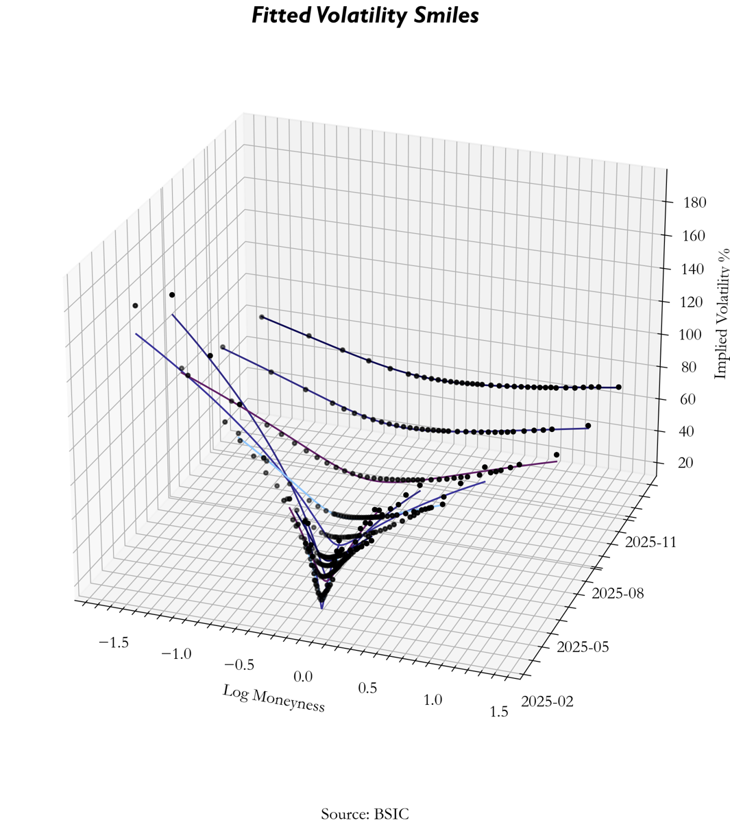
In order to extract the probabilities from option prices it is required to have the IVs for the intermediate strikes, but since not all strike levels are actually traded, we interpolated the implied volatility smile using the available option market data. The volatility smile has been fit using the Stochastic Volatility Inspired (SVI) model for each expiry. The SVI model was introduced by Jim Gatheral as a flexible and arbitrage-free parametric form to describe the implied volatility smile observed in option markets. The (raw) SVI model expresses the total variance $w(k, \tau) \equiv \tau \sigma_{\text{BS}}^2 (k, \tau)$ (where $k = \log\left(\frac{K}{F_{\tau}}\right)$ is the log forward moneyness and $\sigma_{\text{BS}}^2 (k, \tau)$ is the Black-Scholes implied volatility squared) as a function of the form:

$w(k) = a + b \left( \rho (k - m) + \sqrt{(k - m)^2 + \sigma^2} \right)$

Where: $a$ represents the minimum variance level, $b$ controls the overall volatility of the smile, $\rho$ determines the skewness of the smile, $m$ shifts the center of the smile along the strike axis and $\sigma$ adjusts the curvature of the smile.

The parameters of the SVI function must satisfy certain constraints to prevent arbitrage opportunities. In particular the SVI parameters { $a, b, \rho, m, \sigma$ } are such that the resulting volatility curve must not allow for static arbitrage, that is it does not permit butterfly arbitrage and calendar arbitrage. For the sake the reader’s attention span we will not copy-paste the mathematical formulation of the constraints and we will focus merely on the intuition behind the constraint (if you are curious, please check the references for SVI at the end of the article). The first type of arbitrage occurs when an investor can buy a butterfly spread (a structure with non-negative payoffs) for a net credit, thereby locking in risk-free profits. The constraint will be such the investor willing to enter into a fly will pay for it. This, by Breeden-Litzenberger, is equivalent to imposing that the risk-neutral density function is non-negative for every strike level. Instead, the second kind of arbitrage, the calendar arbitrage, occurs when an investor can construct a risk-free calendar spread by shorting a shorter-dated option and going long a longer-dated option at the same $k$ .

Absence of calendar arbitrage is equivalent to saying that call option prices are monotonically increasing as a function of time to maturity, which is also equivalent to imposing that the total variance function $w(k, \tau)$ is monotonically increasing as a function of time to maturity. By fitting the SVI to Deribit implied volatilities we obtained the following output:

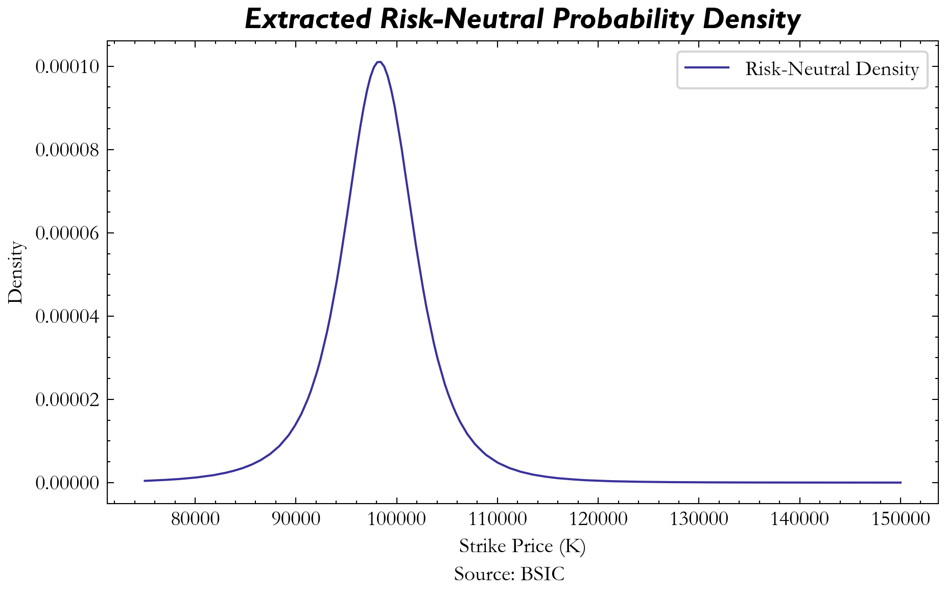
A graph of a graph with lines and numbers AI-generated content may be incorrect.

With an arbitrage-free volatility surface established using SVI, we can now extract the risk-neutral density function $q(K)$ using the Breeden-Litzenberger formula:

$q(K) = \frac{\partial^2 C_{BS} (S_0, K, \sigma(K), r, \tau, q)}{\partial K^2}$

To approximate this second derivative smoothly and avoid numerical instability, we fit a cubic spline to the computed call prices and differentiate it twice, yielding a well-behaved risk-neutral density function.

As previously mentioned, the price a European digital option (cash-or-nothing) is the discounted risk-neutral probability to be above/below the strike at expiration, multiplied by the notional amount. Let’s consider the Kalshi contract that pays 1 USDC if BTC price is above $K$ (European digital call). The risk-neutral probability to be above the strike level at maturity can be computed as

$Q(S_{\tau} \geq K) = \int_{K}^{\infty} q(K) \, dK$

Therefore, the price of the European digital call is:

$p^{\text{digital call}} = Q(S_{\tau} \geq K) \cdot e^{-r \tau} \cdot \textit{Notional}$

Similarly, if we have a European digital put:

$Q(S_{\tau} \leq K) = \int_{-\infty}^{K} q(K) \, dK$

$p^{\text{digital put}} = Q(S_{\tau} \leq K) \cdot e^{-r \tau} \cdot \textit{Notional}$

Finally, we report here the prices of the traded contracts as well as the probabilities we get from our models for the expiry of February 21^st, 2025.

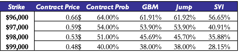
Source: BSIC

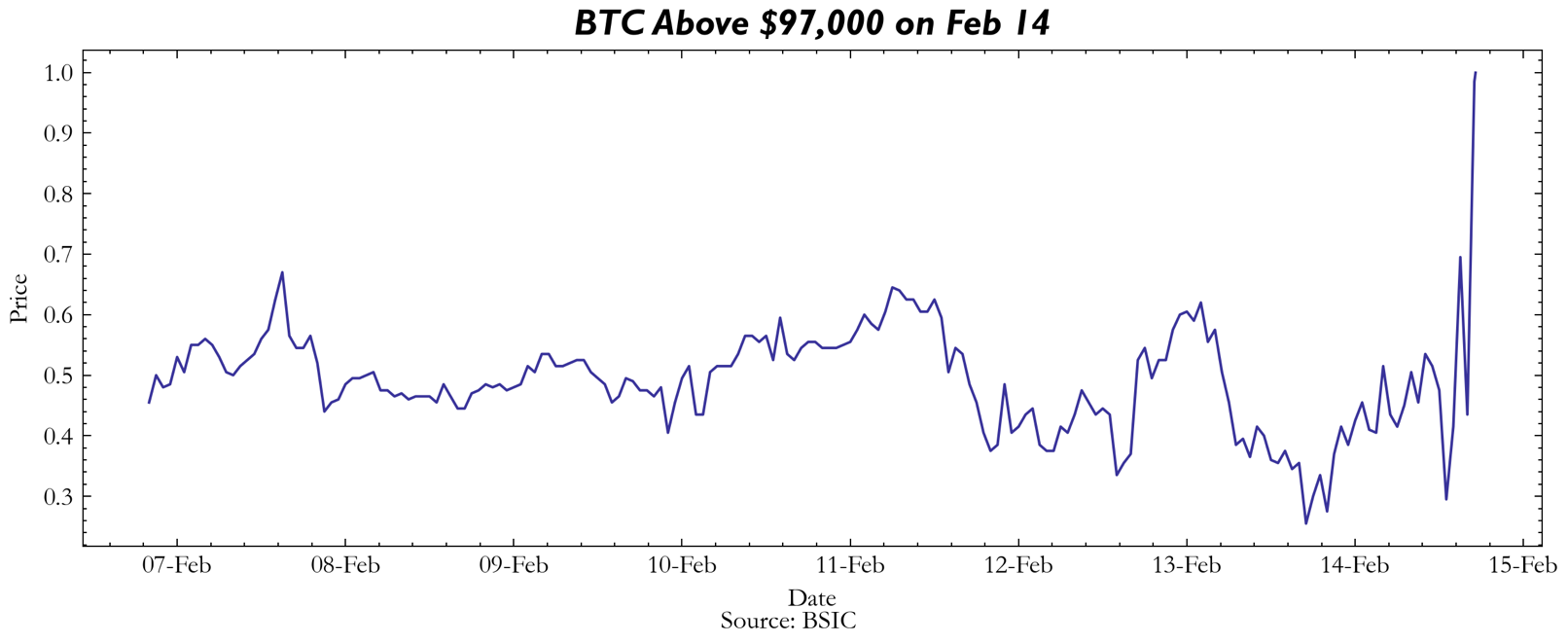
This snapshot was taken at 9PM UTC on February 14^th. Please keep in mind that Kalshi’s contract price-probability differential is representative of the spread that they take between their estimations of probabilities and the fees that they charge (in addition to any other fees). Their reason for inclusion is to gauge if discrepancies exist despite this fee. As can be seen on the table, Kalshi contracts and our GBM models lie within extremely close proximity to one another in terms of probability estimation, while the market IV extracted probabilities lie at a depressed level relative to them, with the biggest deviation being observed at the 99,000 USD strike (roughly 12% differential). Additionally, it’s crucial to note that the time at which we made the table was the same time that Kalshi’s contracts opened, so liquidity was scarce relative to what one would expect on, say, an approximately 3 day-to-expiry option at a given strike. Hence, future analysis needs to analyze how these levels change throughout the maturity of a particular contract.

Conclusion

In this article, we conducted an introductory analysis of crypto prediction contracts and compared different approaches to obtain probability distributions for BTC. Our methodology allowed us to obtain a point-in-time estimate of such distributions to assess whether traded contracts were fairly priced. Our analysis will be expanded upon in the future. Below are some notable considerations regarding the models employed and our findings:

With respect to the GBM with stochastic volatility and jumps added, the benefits are similar. These are computationally efficient stochastic models which incorporate the fat tails needed to adequately measure price fluctuations in BTC. Additionally, computing the parameters such as drift and volatility are relatively straightforward and don’t require much data apart from the BTC price time series. Unfortunately, such parameters lead to potential inaccuracies in approximations across time steps. Since our models used daily price data, these parameters’ estimation loses out on the granularity of BTC’s price action, and in an asset this volatile, intraday data is crucial. Furthermore, our models only make predictions in daily time steps; if a potential prediction contract mispricing doesn’t occur exactly within the indicated time steps, both jump and GBM lose significant predictive power, and adjusting the time steps to make hourly predictions diminishes the robustness of the models due to the data used. In order to improve these stochastic models, intraday data would prove effective, as it would increase the quantity of tradeable strategies that can be explored with reference to the models. Also, the approach for estimating jump intensity and size could be made more robust with the use of a more formal approach such as MLE (maximum likelihood estimation).
For our analysis, we computed the no-arbitrage digital option price by using marked implied volatilities (IV) from Deribit, therefore disregarding how wide the bid-ask spread was, which for crypto options can be quite large due to illiquidity. For instance, on Deribit, the near-ATM contracts typically exhibit bid or ask sizes that rarely exceed one million USD in notional value, which is relatively small by institutional standards. This thin liquidity can impede smooth price discovery and, in turn, introduce problems into the framework. We also weren’t able to find a time series of the IVs at different strikes and maturities, so this made more in-depth analysis quite problematic.
The Deribit contract specifications stipulate that the exercise settlement value (the “fixing”) is calculated using the arithmetic mean of a spot Deribit index over the last 30 minutes before the expiry. This particular calculation is slightly distinct from other digitals, such as Kalshi, where the settlement price is calculated as the mean of a spot BTC index excluding top/bottom 20% values at the 60-second candle during expiry. Naturally, this can introduce problems into inter-exchange strategies which tend to rely on identical methodology to specify exercise value. Additionally, the contracts we considered differ in terms of when they actually expire. Kalshi’s weekly contract expire at 9PM UTC while Deribit’s options expire at 8AM UTC. This would mean that in our last approach is likely underestimating the value of the contracts we considered, as we used risk-neutral probabilities derived from options expiring (13 hours) earlier than the contracts we are supposed to be pricing.

In order to improve this analysis in the future beyond already mentioned considerations, looking at the bid-ask IVs as opposed to marked IVs can help reveal a more detailed view of the market. Additionally, pulling IVs from other large exchanges like Binance or Bybit would provide a better overview of the crypto options market itself. Lastly, a further improvement can be done for our last approach, by calibrating the whole volatility surface (e.g., SSVI), so that we can account for the expiring time discrepancy.

References

Breeden, D. T., and Litzenberger, R. H. “Prices of State-Contingent Claims Implicit in Option Prices”, The Journal of Business, vol. 51, no. 4, 1978
Nielsen S., “The SVI Model – A Tutorial”, 2023
Gatheral J., “A parsimonious arbitrage-free implied volatility parameterization with application to the valuation of volatility derivatives” 2004
Gatheral J., and Jacquier A., “Arbitrage-free SVI volatility surfaces”, 2013

Published by BSIC on 16 February 202516 February 2025

0 Comments

Leave a Reply Cancel reply

Machine Learning Models for S&P 500 Trading: A Comparative Analysis of Random Forest, XGBoost, and Regression Techniques

Market Recap 16/02/2025

Markets X Corporate Finance: Why Domino’s Caught Buffett’s Eye