A Physics – Based Model of Returns: Anomalous Scaling and Irreversibility – BSIC

Abstract

Every empirical study of financial returns since Mandelbrot (1963) has converged on the same short list of stylized facts: heavy polynomial tails, anomalous scaling of volatility with the aggregation horizon, power-law persistence of absolute returns, multiscaling across moment orders, and vanishing linear autocorrelation. These regularities are robust across asset classes, geographies, and decades, yet no single textbook model (Black–Scholes, GARCH, jump-diffusion) reproduces them simultaneously. Each captures one or two features and patches the others, producing an inelegant landscape of model-specific extensions.

We revisit a framework from statistical physics, the Baldovin–Stella (BS) model, originally developed to describe anomalous diffusion in out-of-equilibrium systems throughout phase transitions. Built on a single structural assumption about how memory propagates through returns, the BS model derives the full set of stylized facts as mathematical consequences rather than calibration targets. Its density ansatz is formally identical to Widom’s scaling hypothesis for critical phenomena in Physics; its memory kernel is a fractional integration operator, of the same family underpinning rough volatility and fractional Brownian motion; its time-inhomogeneity encodes the irreversibility of financial evolution in a mathematically precise way.

The article has two aims. The first is to present an elegant, physics-anchored framework for building financial models that account for all the relevant regularities at once, rather than any strict subset. The second is evidential: to argue that the language of statistical mechanics encompassing scaling, universality and irreversibility is not a metaphor but a working toolkit whose financial applications are only beginning to be charted.

Stylized Facts and State of the Art

Each statistical model that aims at reproducing the behaviour and the evolution of financial returns must be calibrated such that the output is consistent with the stylized facts, meaning empirical properties which characterize the distribution of these returns. Before introducing our model, we will briefly summarize these well-known regularities and describe how the latter are expressed and treated in the most famous financial models.

Fat Tails are the expression of extreme returns happening far more often than a Gaussian assumption would allow.
Anomalous scaling of the volatility: empirically, we observe that it deviates of the “square root law” implied by a Standard Brownian Motion
Volatility clustering with long memory: the autocorrelation function of returns decays as a power law not exponentially, translating in persistent fingerprints following shocks.
Multiscaling: the distribution of returns actually changes shape as aggregating across horizons, not just rescale.
Approximately zero linear autocorrelation of returns themselves: today’s returns bear no information about tomorrow market’s behaviour.

Given the generality of these properties, they must constitute the cornerstones of any analytical model for simulating or replicating financial scenarios of this kind, yet standard models usually fall short in incorporating all of these features simultaneously. For example, the renowned Black-Scholes model assumes a Gaussian distribution and cannot exhibit fat tails and clustering; GARCH family models capture volatility clustering but with an exponential decay and does not natively produce power-law memory or multiscaling and, finally, jump diffusions patch fat tails but again fails to model clustering and multiscaling.

In the following sections we will discuss the mathematical foundation of the model and the interpretation of its parameters and then proceed to calibrate the model on a sample containing 130 years of DJIA returns.

Inhomogeneous scaling of the density function

Let’s define $r(t,T)$ as the log-return at time t, aggregated on a scale T and let $p_{T}(r)$ be the pdf of these returns on the same scale. We can now reformulate (SF1-5) in a more formal way:

$p_{T}(r)\, \sim \, C\left| r(t,T) \right|^{- (1 + \alpha)}$ as $|r| \rightarrow \infty$ and $\alpha > 0$
$\sigma(T) = \sqrt{\mathbb{E}\left\lbrack r(t,T)^{2} \right\rbrack}\,\,\sim\, T^{D}$ with $D \neq \frac{1}{2}$
$\mathrm{Corr}\left( \left| r_{t} \right|,\left| r_{t + \tau} \right| \right)\,\sim\,\tau^{- \beta}$ where $0 < \beta < 1$
$\mathbb{E}\left\lbrack \left| r(t,T) \right|^{q} \right\rbrack\sim\, T^{qD(q)}$ with a non-constant $D(q)$
$\mathrm{Corr}\left( r_{t},r_{t + \tau} \right) \approx 0$ for $\tau > 0$

It is worth noting that a standard Gaussian model satisfies only (SF2) with $D = 1/2$ and (SF5), whereas a GARCH model would be able to incorporate also (SF3), albeit with an exponential decay.

In order to create a model which is simultaneously able to meet these requirements and to provide enough degrees of freedom, we make a single strong assumption on the structure of the pdf, which is set to be described by the following expression:

$p_{T}(r) = \frac{1}{\sigma(T)}F\left( \frac{r}{\sigma(T)} \right)$

Where:
$\sigma(T) = T^{D}\, g(t)$

It is now crucial to understand the twofold assumption encompassed in this formalization and to explicit its financial interpretation. Basically, we can disentangle two separate sub-assumptions:

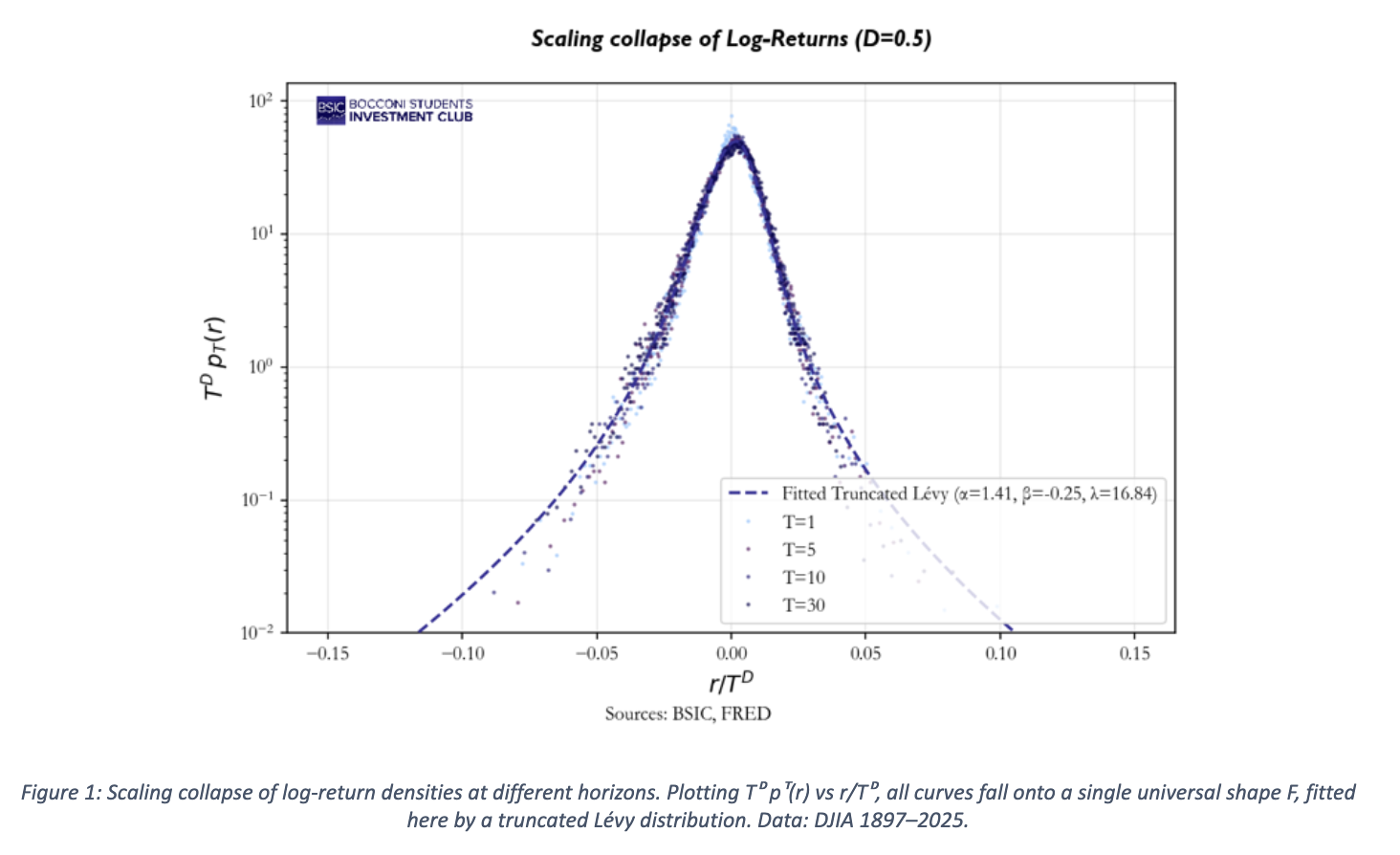
Self-similarity: the pdf on a T horizon is a scaled version of a universal function F. Pragmatically, this means that plotting $\sigma(T)\, p_{T}(r)$ against $r/\sigma(T)$ for different values of T the curves collapse on the single F curve (see Fig.1 below).
Anomalous scaling: the scaling factor is inversely proportional to $\sigma(T)$ , which is, on turn, factored as a power-law and a time-scaling factor g(t).

As it is written, the process is self-affine but not stationary. The introduction of the time scaling factor in the expression for the volatility is crucial, making the model time inhomogeneous. In other words, the explicit presence of the variable t breaks homogeneity and code the irreversibility of the process. The mathematical expression of this function is particularly complex and irrelevant for the purpose of this article, but it models the fact that the markets “ages”, meaning that response change depending on how much time has passed from the initial shock.

The Universal Shape Function: Truncated Levy

We now face the challenge of choosing F such that our (SF1-5) can be satisfied. Of course, the standard Gaussian would fail on fat tails and multiscaling. We opt for a truncated Levy curve: a curve that behaves like a Levy-stable distribution in the middle tails (exhibiting power-law decay), but transitions to Gaussian exponential decay in the extreme tails, ensuring finite variance. We can talk about a “Gaussian-Levy crossover”, modelled by idiosyncratic parameters. This solution is the only one which can simultaneously satisfy the tail, the finite variance and the self-similar scaling requirements. Unfortunately, there exist no simple closed expression for the aforementioned curve, which is indeed often expressed as a characteristic function in the Fourier space, whose specific form is given in the Appendix.

The core idea

In this section our objective is to provide an intuition of the mechanism underlying the model, sufficient to grasp how and why it produces the desired output.

A strong assumption has been made on the marginals of the return distribution at each horizon, but these do not exhaust the description of the stochastic process. We still must specify how returns at different times depend on each other. In very general words, by accounting for the additivity of the log-returns and their non-independence (which along with the scaling ansatz would lead to a Levy-stable process, not suitable for our purpose), the actual process can be described in terms of increments which share some innovations, introducing the desired time-dependence and clustering components.

Delving deeper into this matter, today’s return is computed as a weighted sum of past innovation (i.i.d truncated-Levy), whose weights decay as a power-law. It can be proved (Peirano and Challet, 2012) that, in distribution, the process is equivalent to the following linear filter, where ξ represents the i.i.d shocks and $a_{k}$ the decaying weight of the k-th term (k represents the time “lag”). It is crucial to notice the transition from a family of marginals of the same distribution, to a unique stochastic process, compatible with the required properties.

$\left| r(t) \right| = \sum_{k = 0}^{m} a_{k}\, \xi(t - k)$

The expression for $a_{k}$ is not arbitrary but stems from requiring that the variance scales as $T^{2D_{e}}$ . The explicit formula is now reported for completeness:

$a_{k} = \left\lbrack k^{2D_{e}} - (k - 1)^{2D_{e}} \right\rbrack^{\frac{1}{2D_{e}}}$

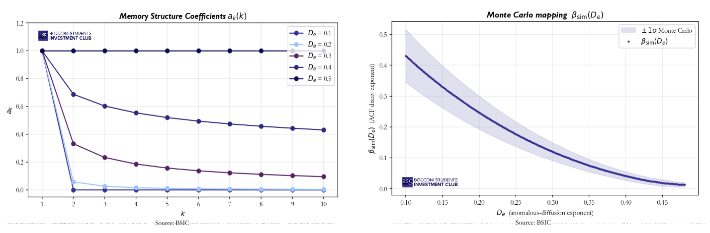
The key parameter is $D_{e}$ , which modules the structure of the memory of the process. We could think of it as the “texture” of the memory kernel, meaning how shocks are distributed across time. Notice how this is fundamentally different from ARMA or GARCH processes, where the exponentially decaying weights allow old shocks to be forgotten within weeks. Low $D_{e}$ means a compressed memory, where only the very recent past matters strongly, though older shocks retain a non-negligible residual. Vice versa, high values of $D_{e}$ mean a flat memory where all past shocks weigh similarly. This latter case converges to the limit of $D_{e} = 1/2$ , which is the pure Gaussian case, in which every past event has the same significance, as well shown in the graph below.

What is now left to explore is the link between the value of this parameter and the empirical distribution. This connection represents the cornerstone of the whole calibration. Asymptotically, the ACF of the absolute returns decays as $\tau^{- \beta}$ and one can show that $\beta = 1 - 2D_{e}$ in the infinite memory, gaussian innovation limit. Practically, finite m, truncated Levy innovations and the time-reset mechanism require a numerical approach. The solution is a Monte Carlo mapping, which simulates the process for a selected array of $D_{e}$ values, estimates $\widehat{\beta}$ for each of them and tabulates the resulting curve. The empirical value of $\beta$ is then inverted trough the curve to yield $\widehat{D_{e}}$ .

In depth look at the Sawtooth Function g(t) and its reset time $\boldsymbol{\tau}_{\mathbf{c}}$

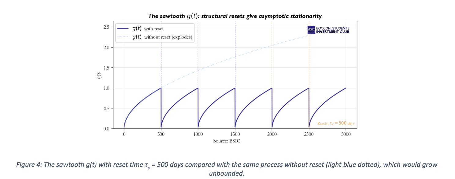
We now return to the time-scaling function g(t). Recall that the model specifies that the scale of log-returns at horizon T depends not only on the horizon itself but also on the absolute time of origin t. It is precisely this dependence that breaks stationarity and makes the process irreversible.

A natural question arises: if g(t) keeps accumulating memory forever, should we not expect the variance of returns to grow without bound over long samples? Empirically, the variance of the DJIA today is not systematically larger than fifty or a hundred years ago, so something must cap this accumulation. The BS model handles this through a structural reset controlled by the reset-time parameter $\tau_{c}$ . Concretely, g(t) grows between successive resets, but every $\tau_{c}$ trading days the clock “restarts” and g(t) returns to its baseline value. The resulting shape is sawtooth.

Summary of the involved variables and parameters

Before delving into the empirical results, it is useful to collect all model parameters and their financial interpretation.

The parameter D measures how quickly the total volatility increases with aggregating horizon. A standard Brownian motion would lead exactly $D = 0.5$ . For different values we talk about super- or sub- diffusion. In very simple terms, whereas normally the monthly volatility turns out being $\sqrt{22}$ times the daily one, here it corresponds to $22^{D}$ times the same benchmark.
$D_{e}$ controls the memory architecture and can be named under effective diffusion exponent. It modulates the weights $a_{k}$ , determining how the past is taken into account in the process. Low values tend to a “Dirac” memory, in which only today’s returns matter, whereas for $D_{e} \rightarrow 0.5$ an homogeneous memory is obtained. Financially, this is the parameter most relevant for pricing path-dependant derivatives and understanding how quickly the market “forgets” a volatility regime.
The exponent $\beta$ measures how quickly the ACF of the absolute returns decays. It is deeply interconnected with the volatility clustering, which gets more evident as the parameter decreases.
The memory is set to be finite and this directly translates into the parameter $m$ , which serves as memory cutoff. In simpler words, it sets after how many trading days the market forgets.
Finally, the hidden parameter $\tau_{c}$ modules the time scaling function g(t) by imposing a structural renewal in the process. Basically, the function g(t) “accumulates” memory for a finite period before being reset and strating over. More formally, our time scaling function represents a sawtooth function which grows between resets, whose frequency is regulated by $\tau_{c}$ . If this limit did not exist, the process could not be asymptotically stationary since g(t) would explode. In financial terms, this assumption makes sure that today’s variance is not systematically higher than fifty years ago, which is empirically evident.

From model to Stylized Facts: Empirical Validation

We calibrate the model on 130 years of DJIA daily returns (1897 – 2025, approximately 32800 trading days). For each stylized fact, we show the empirical evidence, explain which inner mechanism of the model produces it and present the estimated parameters.

Fat tails

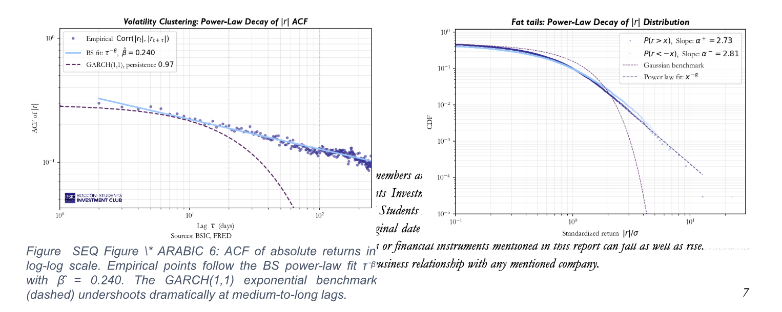
Fig. 5 plots the complementary CDF of standardized absolute returns on a log-log scale. Both the positive and negative tails exhibit the signature of a power law, before tapering off for extreme values. The actual exponent (Pareto exponent) lies well within the range documented in the literature (usually 2 – 5 for equity indices). On the contrary, the Gaussian benchmark clearly fails, falling away far more steeply.

In our model, these fat tails arise because the innovations are drawn from a truncated-Levy distribution, whose tails are polynomial by construction. Underlying this result is another crucial, albeit subtle, aspect. We could be tempted of employing a Central Limit Argument stating that our linear filter will eventually Gaussianise the shocks, which is empirically inaccurate. The pivotal point here is the slow decay of our memory weights, which makes the sum of a finite number of heavy-tailed terms remain heavy-tailed (Generalized Central Limit Theorem).

Volatility Clustering with Power-Law Memory

Fig.6 shows the ACF of the absolute retuns on a log-log scale. The empirical points align on a straight line with slope $- \beta \approx - 0.24$ , confirming power-law decay behaviour over more than two decades of lag. Interestingly enough, the GARCH(1,1) benchmark (persistence 0.97) dramatically undershoots at medium and long lags.

Our linear filter produces absolute returns which share multiple innovations, whose weights $a_{k}$ decay as a power-law, hence the correlation asymptotically tends to this behaviour too. It is worth noticing that the model does not fit the clustering: it predicts it given $D_{e}$ .

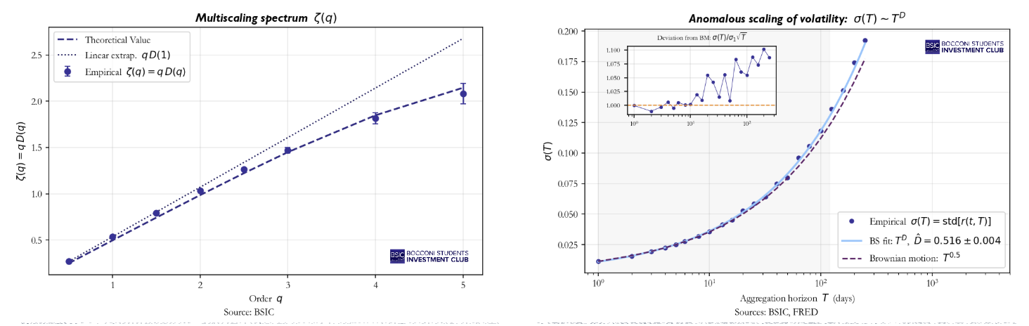
Anomalous Scaling of Volatility

Fig.8 plots the empirical standard deviation of aggregated returns $\sigma(T)$ against the aggregation horizon T on a log-log scale. The fit yields $D = 0.516\, \pm 0.004$ , statistically different form the gaussian benchmark $D_{gauss} = 0.5$ . The inset shows the ratio $\sigma(T)/\left( \sigma_{1}\sqrt{T} \right)$ , which would be constant if diffusion were normal and which shows a statistically significant super diffusion instead.

Multiscaling

Figure 7 shows the scaling spectrum $\zeta(q) = qD(q)$ , empirically estimated from the regression of $\log\mathbb{E}\left\lbrack \left| r(T) \right|^{q} \right\rbrack$ against $\log(T)$ for different moment orders q. If diffusion were purely simple scaling (same exponent for all moments), $\zeta(q)$ would be a straight line through the origin with slope D. Instead, the empirical points curve below this benchmark being strikingly well captured by the mathematical framework of the model. Basically, multiscaling arises because our innovations are characterized by non-trivial higher moments. By aggregating heavy-tailed variables with persistent weights, different moment orders “see” different parts of the tail, producing this moment-dependent scaling. This matters specially for option pricing: non-linearity means that IV across strikes will not obey simple Black-Scholes transformation, giving birth to the well know volatility smile.

Concluding Remarks

The presented framework is valuable not only because of its mathematical elegance, but also because one compact specification produces the five pillars of empirical return behaviour simultaneously. They all emerge from the density ansatz and the very same memory kernel, parametrized by $D_{e}$ and $\beta$ alone. Furthermore, the model offers an ulterior degree of freedom, not addressed by classical models: irreversibility is indeed implemented through the sawtooth function.

Most risk and pricing infrastructures in the financial industry are built on models that explicitly assume away these features. Treating them as core and not as anomalies to patch around may significantly change the perspective about tail risk and pricing. The pivotal parameters of the model emerge as economically meaningful state variables, describing market’s memory architecture. Tracking them down through time may even reveal regime shifts, invisible to simpler classical model.

The broader message of this article aims to be methodological. The language of statistical mechanics turns out to be a real working toolkit to model complex systems even in the financial world, carrying with it a precise, structured but flexible mathematical framework.

From this perspective, financial returns can be naturally interpreted as the “outcome” of a complex system. This opens the door to a deeper form of syncretism between finance and hard sciences, which would encompass the adoption of a full conceptual and technical apparatus, rather than employing just some isolated tools or concepts. In this framework, which is not at all limited to this specific paper, models’ parameters may also be linked to the nature and structural properties of the models themselves, rather than just being considered as calibrations’ outputs.

Mathematical Appendix

Throughout the main body of this article, we have deliberately kept the mathematical details in the background, to favour the communication of the intuition and the empirical validation. Given the general complexity of the theoretical topics, several were introduced only verbally. For completeness, this Appendix aims to provide a deeper insight into these key constructions by filling them in with the minimum rigour to make each step transparent. Nonetheless, we do not attempt a full technical treatment for which one can refer to our references.

The Truncated- Levy Characteristic Function

The universal shape function F is most compactly specified through its Fourier transform, the so-called characteristic function:

$\widetilde{g(k)} \;:=\; \langle e^{ik\xi} \rangle \;:=\; \int F(\xi)\, e^{ik\xi}\, d\xi$

In our specific example we would have:

$\widetilde{g}(k) = \exp\!\left( \frac{- B k^{2}}{1 + C_{a}\, |k|^{2 - \alpha}} \right)$

Effectively, for $|k| \rightarrow 0$ the denominator tends to one and we get the characteristic function for a Gaussian distribution (variance would be equal to 2B). Vice versa, for extreme values of the variable k we get the characteristic function of a Levy-stable curve, whose tails hence decay polynomially:

$\widetilde{g}(k) \;\xrightarrow{\; k \rightarrow \infty \;}\; \exp\!\left( - \frac{B}{C_{a}}\, |k|^{\alpha} \right)$

From Marginal Densities to a stochastic Process

The scaling ansatz we encountered fixes the marginal density of the return $r(t,T)$ at every horizon. However it does not fix the joint distribution of returns at different times, which would be the same as determining the stochastic process itself. It is quite easy to prove that two different processes can have same marginals and yet completely different time-dependence structure.

The requirement that allows to close our construction is the additivity of log-returns, which link returns at different horizons and times:

$r\!\left( t,\, T_{1} + T_{2} \right) = r\!\left( t + T_{1} \right) + r\!\left( t + T_{1},\, T_{2} \right)$

It is now crucial to investigate two possible extreme cases. If the two summands were completely independent, their characteristic function would hence multiply and be consistent with the scaling form:

$\widetilde{p_{T_{1} + T_{2}}}(k) = \widetilde{p_{T_{1}}}(k) \cdot \widetilde{p_{T_{2}}}(k)$

$\widetilde{p_{T}}(k) = \widetilde{g}\!\left( \sigma(T)\, k \right)$

For these to be simultaneously satisfied would force $\widetilde{g}$ to be stable and $\sigma(T)$ to be a simple power, which would fail in reproducing the volatility clustering. Independence is hence incompatible with our empirical sample. In the opposite case, strongly dependent returns would grant volatility clustering but gives birth to an unconstrained problem, that does not fix a unique process.

Our solution sits in the middle of these two extremes. Log-returns are expressed as a sum (integral) of innovations which share support across different horizons. Formally:

$r(t,T) = \sum_{s=0}^{T-1} \left\lbrack \sum_{k=0}^{m} a_{k}\cdot \xi(t + s - k) \right\rbrack$

It is worth noticing that this expression is manifestly consistent with additivity and allows shared innovations and hence some degree of correlation. The work of Peirano and Challet (2012) then provides the key representation result as a linear filter mentioned in the main body of the article.

Derivation of the Memory Weights

Another interesting aspect concerns the structure of the memory weights. They are indeed uniquely determined by the requirements that the variance of aggregated return scales as $T^{2D_{e}}$ . We now explicitly derive the formula. Recalling the linear filter representation of the returns, we can easily compute the aggregated version:

$r(t,T) = \sum_{s=0}^{T-1} r(t + s) = \sum_{s=0}^{T-1} \sum_{k=0}^{m} a_{k}\, \xi(t + s - k)$

Through some algebraic manipulation, the aggregate coefficient ends up being:

$A_{T}(j) = \sum_{k = \max(0,\, t + T - 1 - j)}^{\min(m,\, t - j)} a_{k}$

Now we exploit the fact that these innovations are i.i.d and with fixed variance $\sigma_{\xi}^{2}$ .

$\mathrm{Var}\!\left\lbrack R(t,T) \right\rbrack = \sigma_{\xi}^{2} \cdot \sum_{j} A_{T}(j)^{2}$

We now impose the mentioned scaling requirement:

$\mathrm{Var}\!\left\lbrack R(t,T) \right\rbrack \propto T^{2 D_{e}}\quad\text{for every } T$

Solving this constraint boils down to recognising that the “telescoping” implicit in AT(j) is satisfied by any sequence of the form:

$a_{k} \propto \left\lbrack A(k+1) - A(k) \right\rbrack^{1/2}$

for some function A(·). Imposing the scaling, pins down $A(k) = k^{2 D_{e}}$ which yields:

$a_{k} = \left\lbrack k^{2 D_{e}} - (k - 1)^{2 D_{e}} \right\rbrack^{\frac{1}{2 D_{e}}}$

This is exactly the formula used in the main text. A final technical remark: the formula is valid in the asymptotic, infinite-memory limit and under Gaussian innovations. When the memory is truncated at m and the innovations follow the truncated-Lévy distribution, the relation between $D_{e}$ and the empirical ACF decay exponent β is corrected at finite lags; this is the reason the main text inverts β to recover D̂e via a Monte-Carlo mapping rather than the asymptotic formula β = 1 − 2De.

References

Mandelbrot, B. (1963). The Variation of Certain Speculative Prices. Journal of Business, 36(4), 394–419.
Baldovin, F. & Stella, A.L. (2007). Scaling and Efficiency Determine the Irreversible Evolution of a Market. PNAS, 104(50), 19741–19744.
Baldovin, F. & Stella, A.L. (2007). Central Limit Theorem for Anomalous Scaling. Physical Review E, 75, 020101(R).
Peirano, J. & Challet, D. (2012). Baldovin–Stella Stochastic Volatility Process and Wiener Process Mixtures. European Physical Journal B, 85, 276.
Sokolov, I.M., Chechkin, A.V. & Klafter, J. (2004). Fractional Diffusion Equation for a Power-Law-Truncated Lévy Process. Physica A, 336, 245–251.

A Physics – Based Model of Returns: Anomalous Scaling and Irreversibility

Published by BSIC on 10 May 202610 May 2026

0 Comments

Leave a Reply Cancel reply

Market Recap 10/05/2026

Catching the Butterfly: A Relative Value Approach in OIS Curves

Relative Value in Rates: presenting and challenging the Gauss+ model