Advanced Portfolio Optimization: HRP (Hierarchical Risk Parity)

Download PDF

Introduction

This article explores how Hierarchical Risk Parity (HRP) compares to other portfolio optimization strategies, particularly those based on volatility and traditional portfolio theory. To rigorously test this approach, we constructed a portfolio that rebalances on the first tradable day of December each year from 2005 to 2025.

HRP is an advanced allocation technique that assigns portfolio weights based on volatility to minimize risk. Introduced by Marcos López de Prado in his 2016 paper Building Diversified Portfolios that Outperform Out-of-Sample, HRP was designed as an alternative to conventional risk-based allocation methods, such as Mean-Variance Optimization (MVO) and Risk Parity, Marcos López ended up being the quant of the year. Unlike these traditional models, HRP addresses issues like robustness, numerical instability, and sensitivity to estimation errors.

HRP Breakdown

HRP relies on clustering assets based on returns and assigning weights according to their volatility. Implementing this method requires three key steps:

1. Hierarchical Clustering

2. Quasi-Diagonalization

3. Recursive Bisection

HRP provides a robust alternative to conventional allocation methods by structuring a portfolio in a way that aligns more naturally with how assets behave in the real world. To evaluate its effectiveness, we conducted a backtest from 2005 to 2015, using a dataset of approximately 1,292 U.S. stocks. This long testing period ensures a fair assessment, as shorter timeframes could introduce misleading conclusions.

However, eliminating biases from historical data is never a straightforward task. Many portfolio strategies that appear to “outperform” are often unintentionally engineered to reflect past trends rather than offering a truly robust framework for future returns. One of the most common biases is the momentum effect, leading many allocation models to overweight tech stocks, particularly in recent years, but this is just a bias because we already know, how last year’s stock market developed. Since HRP does not rely on factor-based selection, our goal was to avoid any artificial performance enhancement caused by sectoral biases.

To further ensure fairness in our analysis, we implemented a consistent rebalancing rule: every first tradable day of December. This choice is not totally arbitrary; it is inspired by the December Effect, which accounts for tax-loss harvesting behavior and year-end portfolio adjustments by institutional investors. In essence, December serves as a natural rebalancing period in real-world trading, making it a practical and applicable rule for long-term portfolio management.

Now, let’s break down each step of the HRP process.

Hierarchical Clustering

Hierarchical clustering is the first step in HRP, grouping assets into clusters based on their return correlations. This begins with calculating a correlation matrix, followed by a distance matrix, which quantifies how similar or different the assets are. In order to do that we start by calculating the correlation matrix between our stocks, from which then we compute the distance matrix, with the correlation distance formula:

where   is the Pearson coefficient (correlation coefficient) and represents the distance, the one we want to calculate it.

To measure the distance between assets, we employ various linkage methods, which define how clusters are formed based on distance metrics. Some commonly used techniques include single linkage, complete linkage, average linkage, and Ward’s linkage. Among these, average linkage and Ward’s linkage are particularly effective. Average linkage calculates the mean distance between points in different clusters, while Ward’s linkage measures the increase in squared error when two clusters merge. In our methodology, we utilize average linkage for clustering assets and Ward’s linkage for determining HRP portfolio weights.

A fundamental question in clustering is determining the optimal number of clusters. Running multiple clustering models is computationally expensive, so we employ an evaluation technique known as the Silhouette Score to assess clustering effectiveness. The evaluation model works in the following way: is a measure of how well-separated clusters are, ranging from -1 to +1. A score close to +1 indicates that a point is well clustered and far from other clusters, while a score of 0 suggests that the point is on the decision boundary between two clusters. Then we calculate   and   , respectively intra-cluster distance and nearest-cluster distance, for each data point (info about how to calculate these two parameters is going to be in the references). Once we have these two parameters then we calculate the Silhouette Coefficient for each data point with the following formula:

And then finally we can assign the Silhouette Score by computing the average of individual scores across all points in the dataset.

As it’s clear from the chart the best number of clusters in this case in 2, so that’s what the model will interpret as number of clusters. Once the number of clusters is determined and the distance matrix is computed, we visualize the clustering process using a Dendrogram, a hierarchical tree representation of asset groupings. In this visualization, the x-axis represents individual stocks, while the y-axis corresponds to the calculated distances.

Quasi – Diagonalization

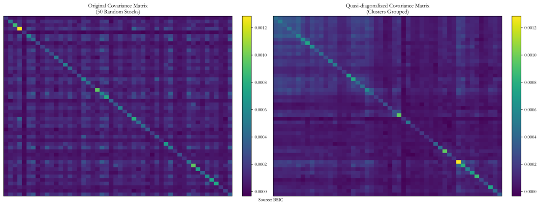
In the second step of the HRP process, we refine the covariance matrix of the assets by applying quasi-diagonalization. This step involves calculating the covariance between each pair of assets and then reorganizing the rows and columns of the covariance matrix so that assets with similar return patterns are grouped together, while those with weaker correlations are placed farther apart.

By rearranging the covariance matrix in this manner, the most significant covariance values are concentrated along the diagonal, while smaller values are dispersed. This transformation enhances the portfolio’s ability to allocate risk effectively, reducing the impact of highly correlated assets on overall volatility.

Recursive Bisection

The most important part of HRP (Hierarchical Risk Parity) is how it assigns weights to assets. The process follows a top-down, recursive approach. Unlike Mean-Variance Optimization (MVO), introduced by Harry Markowitz, which assigns weights simultaneously to all assets by solving an optimization system balancing expected return and risk, HRP begins with the entire portfolio as a single cluster and progressively breaks it down into smaller sub-clusters based on a hierarchical tree structure.

The key idea is that once the quasi-diagonalized covariance matrix is structured, HRP proceeds by splitting the largest cluster into smaller clusters. It moves down the hierarchy step by step, breaking each cluster into two sub-clusters at each stage. This process continues until all individual assets are assigned a weight.

HRP follows a risk-based approach, assuming that if the covariance matrix were perfectly diagonal (i.e., assets were completely independent), the inverse-variance allocation would be the best way to distribute weights. In simple terms, this means that less volatile assets receive higher weights, while riskier assets get lower weights. By applying this logic recursively at each step, risk is efficiently allocated within each cluster before moving further down the hierarchy.

This approach minimizes concentration risk in any single asset or group. Instead of relying on traditional methods like Markowitz’s MVO, which can be highly sensitive to estimation errors, HRP constructs a more stable and diversified portfolio by respecting the natural structure of asset returns and relationships.

Data

We have collected data from February 11, 2005, to February 26, 2025, covering approximately 3,000 U.S. stocks. Since cleaning such a large dataset would be time-consuming, we decided to focus only on stocks that have been continuously listed from 2005 to 2025.

At first glance, this selection might seem biased, as it excludes delisted or defaulted stocks while also ignoring newer stocks that have entered the mid- or high-cap segment after 2005. However, our rationale is that by focusing on long-standing stocks, we avoid the downside risk of selecting companies that have failed, while also missing out on new opportunities that have emerged in the market. After filtering, we narrowed the dataset from 3,000 stocks to approximately 1,500. On these stocks, we constructed two equally weighted portfolios: one that we decided to rebalance every December, and one which is not rebalanced. For benchmarking, we included the S&P 500 index.

Results

We start with a simple plot comparing the Equally Weighted (Rebalanced and Non-Rebalanced) Portfolios and the S&P 500. From the chart, it is evident that the non-rebalanced portfolio significantly outperforms both the S&P 500 and the rebalanced portfolio. This is due to the fact that not rebalancing in a high-momentum market (such as the last 20 years, except for 2008) benefits a buy-and-hold strategy. However, concluding that non-rebalancing is always superior would be misleading. The outperformance is likely due to the specific market conditions over the examined period, where momentum was strong. In different market conditions, rebalancing could provide better risk-adjusted returns. Nevertheless, a key takeaway is that both the rebalanced and non-rebalanced portfolios have outperformed the S&P 500.

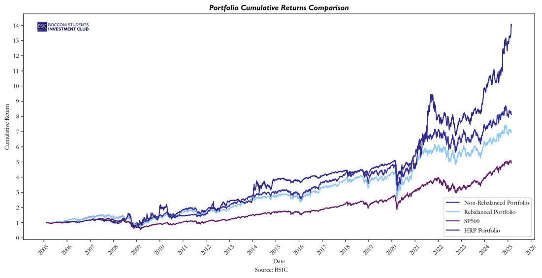
Now, let’s analyze how HRP performed compared to the three other portfolios.

The results demonstrate an exceptional performance by HRP relative to the broader market, achieving a cumulative return of 1,299.67%. However, despite its strong returns, the drawdown metrics reveal significant risk, as HRP experienced a maximum drawdown of -60% during the 2008 financial crisis.

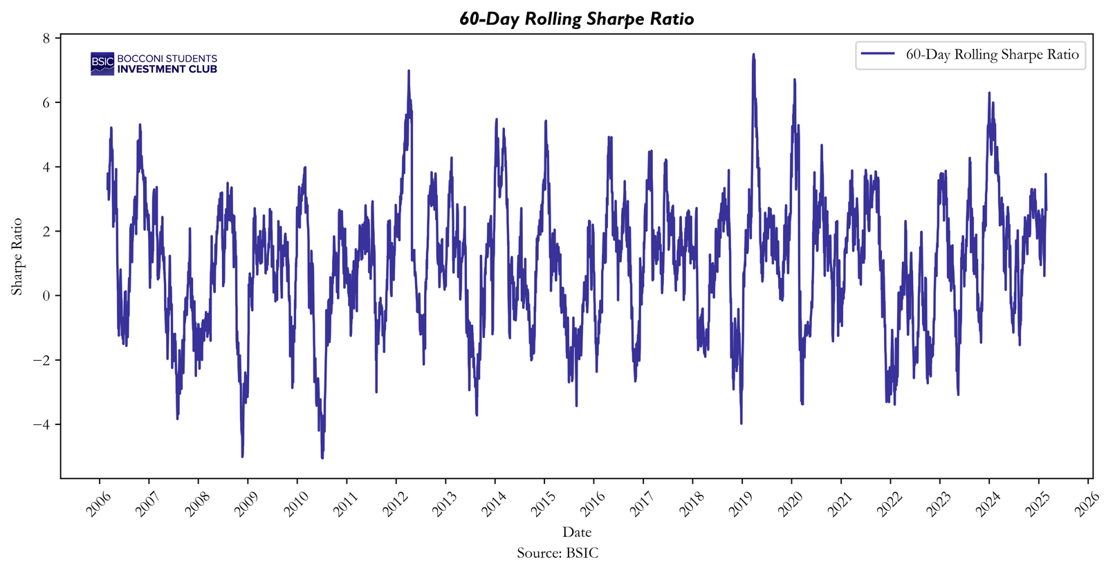Regarding risk-adjusted returns, the mean Sharpe ratio stands at 0.4711, with a standard deviation of the rolling Sharpe ratio (calculated using a 60-day time window) of 1.9575. This indicates that while HRP delivers high returns, its risk-adjusted performance is relatively volatile over time.

References

[1] Aditya, Vias, “The Hierarchical Risk Parity Algorithm: an Introduction”, 2020