An Estimation of the Risk Premium as Function of the VIX

Introduction

The expected excess market return, or equity risk premium, is an unobservable element crucial in many financial applications ranging from corporate finance to asset pricing. Over the years, many researchers have studied the expected market return by tackling the estimation from different perspectives leading Welch, Goyal (2008) and Campbell, Thompson (2008) to re-examine the performance of such indicators from a common standpoint.

In the academic literature, the traditional predictors of the expected returns have been documented to be valuation ratios such as: dividend-price ratio, dividend yield, earnings-price ratio, or book-to-market ratio. More recently, Chabi-yo, Loudis (2019) suggests a different approach: the equity premium can be reliably quantified by conditional risk-neutral moments of excess market returns.

In this article, we take the Chabi-yo, Loudis (2019) lower bound on the conditional expected return as given, inviting the most curious readers to examine the original paper further, and solve an inherent practical problem of their work: the high computational intensity of the estimation. In fact, while the two authors use the Carr, Madan (2001) spanning formula in order to write risk-neutral moments in terms of option prices, we show how to simplify the process by approximating risk-neutral moments through functions of the VIX, a readily available index published by the Chicago Board Options Exchange.

Chabi-Yo, Loudis (2019) Lower Bound on the Conditional Excess Expected Market Return

Chabi-yo, Loudis (2019) lower bound is expressed as:

$LBR_{t\rightarrow T}=\frac{\sum_{k=1}^{3}\frac{\left(-1\right)^{k+1}}{R_{f}^{k}}\mathbb{M}_{(k+1)}^{*}}{1+\sum_{k=2}^{3}\frac{\left(-1\right)^{k+1}}{R_{f}^{k}}\mathbb{M}_{(k)}^{*}}$

where $\mathbb{M}_{(k)}^{*}$ stands for the conditional risk-neutral n-th excess moment:

$\mathbb{M}_{(n)}^{*}=E_{t}^{*}\left[\left(R_{m}-R_{f}\right)^{n}\right],\,\,\,\,\,\,\,\,\,\,n>0$

and $R_{m}, R_{f}$ for the market gross return and risk-free rate from t to T, where gross return is simply defined as $S_{T}/S_{t}$ .

Lower Bound as Function of the VIX Index

According to its white paper, the VIX index is defined as the annualized risk-neutral expectation of integrated variance over the next 30 days:

$VIX_{t}^{2} =\frac{1}{T-t}E_{t}^{*}\left[\int_{t}^{T}\sigma_{\tau}^{2}d\tau\right]=\left(\sigma_{t}^{T}\right)^{2},\,\,\,\,\,\,\,\,\,\,T=t+30\text{ days}$

In order to measure the VIX, the Cboe expresses the risk-neutral expectation in terms of a function of $S_{t}$ , namely the logarithm.

By assuming a stock evolution process in the form of diffusion on the risk-neutral probability space $\left(\Omega,\mathbb{F},\pi^{*}\right)$ :

$dS_{t}=r_{t}S_{t}dt+\sigma_{t}S_{t}dW_{t},\,\,\,\,\,\,\,\,\,\,S_{0}=s_{0}$

where $r_{t}$ and $\sigma_{t}$ , respectively drift and volatility coefficients, are deterministic functions of time t; and $W_{t}$ is a standard Brownian motion on the same probability space. We apply Ito’s lemma to obtain the stochastic differential equation (SDE) of the log-contract:

$d\ln S_{t}=\left(r_{t}-\frac{1}{2}\sigma_{t}^{2}\right)dt+\sigma_{t}dW_{t},\,\,\,\,\,\,\,\,\,\,\ln S_{0}=\ln s_{0}$

By taking the risk-neutral expectation of the integrated logarithm, we obtain:

$\begin{aligned}E_{t}^{*}\left[\int_{t}^{T}d\ln S_{\tau}\right]=E_{t}^{*}\left[\int_{t}^{T}\left(r_{\tau}-\frac{1}{2}\sigma_{\tau}^{2}\right)d\tau+\int_{t}^{T}\sigma_{\tau}dW_{\tau}\right]\\E_{t}^{*}\left[\ln\frac{S_{T}}{S_{t}}\right]=r_{t}^{T}\left(T-t\right)-\frac{1}{2}E_{t}^{*}\left[\int_{t}^{T}\sigma_{\tau}^{2}d\tau\right]\\-2E_{t}^{*}\left[\ln\frac{S_{T}}{F_{t}^{T}}\right] =E_{t}^{*}\left[\int_{t}^{T}\sigma_{\tau}^{2}d\tau\right]\\-\frac{2}{T-t}E_{t}^{*}\left[\ln\frac{S_{T}}{F_{t}^{T}}\right] =VIX_{t}^{2}\end{aligned}$

with $F_{t}^{T}=S_{t}R_{f}$ . For our purposes, we are interested in using the VIX as an estimator of the risk-neutral expectation of log-return, thus we will be using the second line of the previous block of equations:

$E_{t}^{*}\left[\ln R_{m}\right]=r_{t}^{T}\left(T-t\right)-\frac{1}{2}VIX_{t}^{2}\left(T-t\right)$

Under an assumption of log-normality of stock returns, also the risk-neutral 2nd return moment can be expressed as a function of VIX.

$\begin{aligned}E_{t}^{*}\left[R_{m}^{2}\right] =E_{t}^{*}\left[e^{2\left[\int_{t}^{T}\left(r_{\tau}-\frac{1}{2}\sigma_{\tau}^{2}\right)d\tau+\int_{t}^{T}\sigma_{\tau}dW_{\tau}\right]}\right] \\ =e^{2r_{t}^{T}\left(T-t\right)-\int_{t}^{T}\sigma_{\tau}^{2}d\tau}E_{t}^{*}\left[e^{\int_{t}^{T}2\sigma_{\tau}dW_{\tau}}\right]\\ =e^{2r_{t}^{T}\left(T-t\right)-\left(\sigma_{t}^{T}\right)^{2}(T-t)}e^{0+\frac{1}{2}\left[4\left(\sigma_{t}^{T}\right)^{2}\left(T-t\right)\right]}\\ =R_{f}^{2}e^{\left(\sigma_{t}^{T}\right)^{2}(T-t)},\,\,\,\,\,\,\,\,\,\,\left(\sigma_{t}^{T}\right)^{2}=VIX_{t}^{2}\end{aligned}$

where on the third line we take the expectation of the exponential of the stochastic integral $\int_{t}^{T}2\sigma_{\tau}dW_{\tau}$ which has mean $0$ and variance $4\left(\sigma_{t}^{T}\right)^{2}\left(T-t\right)$ .

In order to approximate risk-neutral expectation of excess returns, we first decompose them into returns by breaking down the binomials. For example, for the 2nd excess moment we obtain:

$\begin{aligned}E_{t}^{*}\left[\left(R_{m}-R_{f}\right)^{2}\right]=E_{t}^{*}\left[R_{m}^{2}\right]+R_{f}^{2}-2E_{t}^{*}\left[R_{m}\right]R_{f}\\ =E_{t}^{*}\left[R_{m}^{2}\right]-R_{f}^{2}\end{aligned}$

where the risk-neutral expectation of gross return is the risk-free factor.

Then, we proceed by following the intuition of Bakshi, Kadapia, Madan (2003): the expectation of the gross return, $R_{m}$ , can be decomposed into expectation of log-returns through a Taylor expansion on $f\left(\ln R_{m}\right)=e^{\ln R_{m}}=R_{m}$ around $\ln R_{m}=0$ . In addition, such intuition can be applied to all powers of gross returns.

In general, let $x=\ln R_{m}$ be our independent variable, and $f(x)=e^{nx}$ be our function of interest; by taking the Taylor expansion around $x_{0}=0$ , and up to the 3rd order, we obtain:

$e^{nx} =1+nx+\frac{1}{2}n^{2}x^{2}+\frac{1}{6}n^{3}x^{3}+o\left(x^{4}\right)$

by writing the equation in terms of gross returns $R_{m}$ and taking its risk-neutral expectation:

$e^{nx}=1+nx+\frac{1}{2}n^{2}x^{2}+\frac{1}{6}n^{3}x^{3}+o\left(x^{4}\right)$

Then, we observe that some of the terms within this equation are already known: $E_{t}^{*}\left[R_{m}\right]$ is equal to the risk-free factor, $E_{t}^{*}\left[\ln R_{m}\right]$ and $E_{t}^{*}\left[R_{m}^{2}\right]$ are both functions of VIX. Thus, by solving a system of 2 equations above (for n=1,2) with 2 unknowns allows us to find, first, the missing log-return moments, and then the interested return moments (for n=3,4).

$\begin{cases}E_{t}^{*}\left[\left(\ln R_{m}\right)^{2}\right]=\frac{1}{2}\left[8R_{f}-6E_{t}^{*}\left[\ln R_{m}\right]-E_{t}^{*}\left[R_{m}^{2}\right]-7\right]\\E_{t}^{*}\left[\left(\ln R_{m}\right)^{3}\right]=\frac{3}{2}\left[-4R_{f}+2E_{t}^{*}\left[\ln R_{m}\right]+E_{t}^{*}\left[R_{m}^{2}\right]+3\right]\end{cases}$

The last step remains to reconstruct the binomials of excess return from return moments.

Application to the US Market

In the previous section, we demonstrated that the Chabi-yo, Loudis (2019) lower bound can be replicated efficiently by a function of the VIX index. This allows practitioners to quickly obtain an estimate of the conditional expected market return which can be computed at daily or even higher frequency.

In this section, we apply such methodology on the US market, proxied by the S&P 500 index. While the 30d risk-free rates are obtained from OptionMetrics, the SPX and VIX indices are obtained from Bloomberg. The sample period runs from 1st Jan 1996 to 31st Dec 2018.

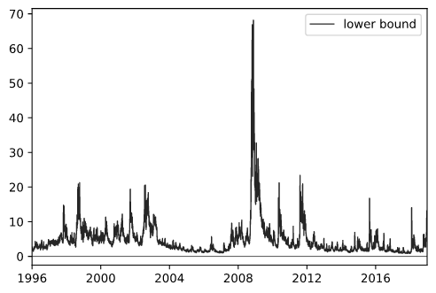
Figure 1: Lower bound of the conditional expected market return, in annualized and percentage terms.

In figure 1 we plot the time-series of the replicated 30d lower bound (annualized and in percentage terms), which can be seen to be highly volatile and tends to spike during periods of economic stress.

In order to show that such bound is a good predictor of the risk premium, we run an OLS forecasting regressions of the following form:

$R_{m,t\rightarrow T}-R_{f,t\rightarrow T}=a+bLB_{t\rightarrow T}+\epsilon$

In addition, we compute the out-of-sample $R^{2}$ of Welch, Goyal (2008) and Campbell, Thompson (2008) by following the predicting expanding window regression of Ferreira, Santa-Clara (2011). In their paper, they explain how they simulate what a forecaster could have done in real time.

Specifically, we set the out-of-sample date as $s_{0}=31^{st}$ Dec 2016, i.e. 2 years before the end of sample. Next, we split the sample into 2 sub-groups: an expanding in-sample of $t=1,2,...,s$ and contracting sample of $t=s+1,s+2,...,S$ with the varying end-point $s\in\left[s_{0},S\right]$ . Note the difference between $T=t+30d$ and $S$ being the last date in our sample, i.e. $31^{st}$ Dec 2018.

Using the in-sample observations, we estimate forecasting regression to obtain a forecast for $t=s+1$ as conditional expectation:

$\hat{E_{s}\left[R_{m,s+1}-R_{f,s+1}\right]}=\hat{a}_{s}+\hat{b}_{s}x_{s}$

where we denote with the subscript $s$ the estimated parameters of the forecasting regression with the sample up to $s$ .

Such estimators are compared against the historical excess mean model estimated through the difference between the geometric average return of the market and of the risk-free rate from CRSP beginning in 1926.

Finally, we measure the forecasting performance of our variable against the historical sample mean using the out-of-sample $R^{2}$ computed according to:

$R_{OOS}^{2}=1-\frac{MSE_{A}}{MSE_{N}}$

where $MSE_{A}$ is the mean square error from the predicting regression and $MSE_{N}$ from the historical mean model:

$MSE=\frac{1}{T}\sum_{s=1}^{T}\left(Y_{s}-\hat{Y}_{s}\right)^{2}$

It must be stated that while the standard $R^{2}$ can take values from 0 to 1, the out-of-sample one can take negative values. This happens when the $MSE_{N}<MSE_{A}$ , i.e. the historical mean model predicts better than the interested regression.

Table 1: Regression results of the lower bound on the historical excess market return, annualized for the period starting 1st Jan 1996 to 31st Dec 2018, with an out-of-sample starting date of 31st Dec 2016. The historical mean model for the out-of-sample $R^{2}$ uses information from Jan 1926.

Table 1 reports the result of such approach. From it, we can notice that the intercept and slope coefficient cannot be rejected to be statistically different from 0, 1. It entails that the bound is fairly tight.

The out-of-sample $R^{2}$ statistic of 0.88% shows promising result, especially if compared with the findings of Welch, Goyal (2008) which test many conventional predictor variables as such: dividend-price ratio, dividend yield, earnings-price ratio, book-to-market ratio and obtain negative out-of-sample $R^{2}\text{ of} -2.06\%, -1.93\%, -1.78\% \text{ and} -1.72\%$ respectively.

References

Chabi-Yo, Fousseni, and Johnathan Loudis. The Conditional Expected Market Return. Journal of Financial Economics (JFE) 10 Jul 2019.

References Carr, Peter, and Dilip Madan. Optimal Positioning in Derivative Securities. Journal of Quantitative Finance Vol. 1, Issue 1, 2001: pp: 19-37.

References Welch, Ivo, and Amit Goyal. A Comprehensive Look at the Empirical Performance of Equity Premium Prediction. The Review of Financial Studies Vol. 21, Issue 4, July 2008: pp. 1455-1508.

References Campbell, John Y., and Samuel B. Thompson. Predicting Excess Stock Returns Out of Sample: Can Anything Beat the Historical Average? The Review of Financial Studies Vol. 21, Issue 4, July 2008: pp. 1509-1531.

References Bakshi, Gurdip, Kapadia, Nikunj, and Dilip Madan. Stock Returns Characteristics, Skew Laws, and the Differential Pricing of Individual Equity Options. The Review of Financial Studies Vol. 16, Issue 1, January 2003, pp. 101-143.

References Ferreira, Miguel A., and Pedro Santa-Clara. Forecasting Stock Market Returns: The Sum of the Parts is More than the Whole. Journal of Financial Economics Vol. 100, Issue 3, June 2011: pp. 514-537.

Published by BSIC on 10 May 202010 May 2020

0 Comments

Leave a Reply Cancel reply

Corporate Finance Markets

Exploring the Practicality of Merger Arbitragе

Markets

Market Recap 05/05/2024

Markets

A Systematic Approach to Credit Investing

An Estimation of the Risk Premium as Function of the VIX

Published by BSIC on 10 May 202010 May 2020

0 Comments

Leave a Reply Cancel reply

Related Posts

Corporate Finance Markets

Exploring the Practicality of Merger Arbitragе

Markets

Market Recap 05/05/2024

Markets

A Systematic Approach to Credit Investing