The Low-Beta Anomaly
The Low-Beta Anomaly is a well-documented stock market anomaly in which low beta stocks outperform high beta stocks. This goes against what basic financial intuition and theory would suggest; most notably it stands in direct opposition to the Capital Asset Pricing Model which stipulates that the return of stocks is a function positively dependent on beta. First documentations of this anomaly range back to the 1970s and subsequent research has found a consistent abnormal return associated to low beta stocks until this day. To illustrate, the below chart shows a comparison of the returns of U.S. stocks when sorted by their beta.
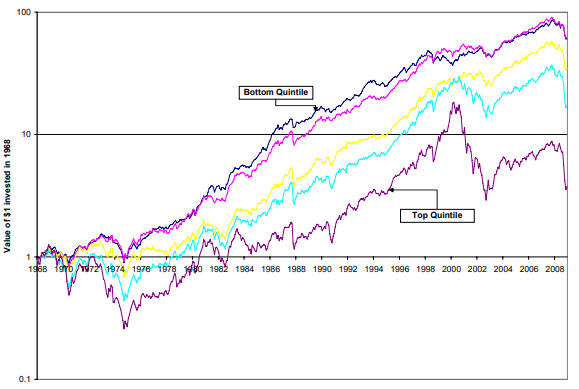
Source: [2]
To take advantage of this phenomenon, multiple approaches can be taken, all of which can be classified as either taking a long position in low-beta stocks or taking a short position in high-beta stocks or combining the previous two approaches. A word of caution should be spoken here. As is shown by research conducted by Korn and Kuntz, depending on how one chooses to compare different stocks according to their beta, vastly different results can be obtained. Take the following figure as an example.
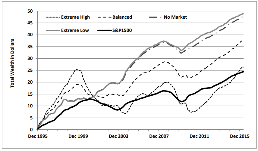
Source: [1]
The “Extreme High” strategy takes only a short position in high-beta portfolios while the “Extreme Low” strategy takes only a long position in low-beta portfolios and both the “Balanced” and “No Market” strategies take both long and short positions respectively differing only in the fact that the former strategy invests the same nominal amounts in each portfolio while the latter invests amounts weighted by the betas of the high- and low-beta portfolios. Evidently, there are large differences in the performance of the different strategies; however, all studies highlighted in this article use a method that exclusively goes long on low-beta stocks, so subsequent analysis will refer to this strategy. However, changing other variables when constructing the beta-sorted portfolios also has a substantial impact on the performance of the strategy. Most importantly, the weighting of single stocks within the portfolios and the choice of an investment universe affect performance: 1. with an investment universe of the S&P 1500, value weighting has lower alpha than equal weighting which has lower alpha than beta weighting and 2. shrinking the investment universe from the S&P 1500 to S&P 500 while applying beta weighting reduces alpha so drastically that it is not statistically relevant anymore. Therefore, we have checked the investment universe and weighting used for the papers that are used.
Because financial theory could not explain the Low-Beta Anomaly, numerous explanations in the field of behavioral finance have been put forward. This article will compare three of them and discuss what an investor should pay attention to, when trying to exploit this anomaly.
Benchmarks as Limits to Arbitrage
The first study is a great resource for anyone who wants to start getting to know more about behavioral finance, as it uses three of the most well-known behavioral finance phenomena to explain parts of the Low-Beta Anomaly.
In the first part of their explanation, the authors name two irrationalities of retail investors that could contribute to the Low-Beta Anomaly. Sadly, they do not provide rigorous tests for these explanations. Nevertheless, the paper can be used as a source for the intuition behind the Low-Beta Anomaly which is expanded upon in the subsequent sections.
The first phenomenon that is drawn upon is the preference for so-called lottery-stocks by retail investors. As is the case in lotteries, the payoff of investing in highly volatile stocks exhibits positive skewness, meaning investors have a small chance of gaining large but on average will lose money. The preference of retail investors for this type of stocks is a classic example of longshot bias, where investors are overly optimistic towards winning big which drives up prices of high-beta stocks, in turn reducing their returns over the long run. The authors stipulate that this bias is a consequence of a representativeness issue, more specifically the conjunction fallacy. By this fallacy, retail investors are more inclined to invest in very volatile stocks which are seen as ‘great investments’ since many of the most profitable investments have been associated to volatile stocks. What investors overlook however, is that volatile stocks only make up a subset of the category of ‘great investments’. In other words, investors falsely assign a higher subjective probability to the statement “a stock is highly volatile and a great investment” than to “a stock is a great investment” which overly increases demand for lottery-stocks.
Secondly, the authors mention overconfidence in one’s predictions as a reason for the Low-Beta Anomaly. The reasoning goes as follows: For highly volatile stocks, disagreement between stock price predictions of optimists and pessimists is greater than for less volatile stocks and since stock prices are primarily influenced by optimists, highly volatile stocks are bid up which reduces returns.
What clearly follows from these explanations is the question of why this anomaly is so persistent over time, even though it is very well documented. In other words, even though retail investors have these biases, why haven’t institutional investors taken advantage of them? The obvious answer is that there must be some kind of limit to arbitrage – the authors propose that benchmarking could be such a limit.
Benchmarking is a common practice for institutional investors in which the returns of a portfolio manager are compared to a benchmark. A ratio that is often used is the so-called information ratio which is defined as  , with the Tracking Error being defined as the standard deviation of the numerator. Assuming a portfolio manager wants to overweight a low-beta
  stock with a higher expected return than the market in an otherwise market-portfolio by a fraction
  , in a CAPM-framework there are two opposing effects on the numerator of the information ratio which are captured by the following formula:
  . Here, represents the excess return of the low-beta stock, while
  represents the negative impact of that stock on the expected return of the portfolio. This means that
  must hold in order for the information ratio to increase. The opposite is true for high-beta
  stocks: the underperformance of these stocks has to be sufficiently large in order to decrease the overall expected return of the portfolio. In practice, this discourages portfolio managers from taking advantage of the Low-Beta Anomaly – in other words, benchmarking contributes to the persistence of the Low-Beta Anomaly.
Demand for Lottery-Stocks
The hypothesis of investors bidding up lottery-like stocks is explored further in paper [3]. In their investigations, they use a large sample space of all U.S. stocks with stock prices above $5 in the CRSP database and use equal-weighting in the beta-sorted portfolios. Their measure for lottery-demand for a given stock is calculated as the average of the five highest daily returns of that stock during the previous month with higher averages indicating higher demand for lottery-stocks. This measure was proposed by the authors in a previous paper as a robust measure for lottery-demand.
The authors find that when controlling for the effect of a higher than usual lottery demand, the Low-Beta Anomaly disappears while it did not disappear when controlling for other firm characteristics and risk measures, indicating that demand for lottery-like stocks is an important reason for the Low-Beta Anomaly. What is more, the authors confirm the hypothesis that high-beta stocks exhibit lower returns due to the fact that they are bid up by individual investors looking to invest in lottery-like stocks. Namely, they find that high-beta stocks are disproportionately affected by price pressure stemming from demand for lottery stocks and that the Low-Beta Anomaly predominantly appears in stocks which are held by individual rather than institutional investors. The latter observation somewhat contradicts the notion that the Low-Beta Anomaly persists due to benchmarking being a limit to arbitrage for institutional investors; rather, there have to be more effects at play which are not yet uncovered.
Beta Herding through Overconfidence
Paper [4] investigates overconfidence as an explanation for the Low-Beta Anomaly further. The authors use an investment universe of all stocks traded on the NYSE, AMEX and NASDAQ with market capitalizations in the top 80% and value-weight their portfolios. The theoretical foundation in a CAPM framework for overconfidence is outlined as follows (please note that overconfidence refers to overconfidence in the precision of signals about the market outlook):
When investors receive a signal to predict market return, they update their posterior expectation of the market return accordingly – if these investors are overconfident in the precision of that signal, they overreact to it and buy or sell shares such that the betas of individual stocks are compressed towards the market beta which is referred to as beta herding. If they are underconfident, the opposite happens, and the betas of individuals stocks are dispersed away from the market beta which is referred to as adverse beta herding. In turn, over- and underconfidence also affect expectations of market return which is illustrated by different shifts in the Security Market Line (SML). As is shown in the graph below, when starting from the thin blue line in the middle as a base case scenario, the SMLs for underconfident investors shift too little when receiving a positive or negative signal about market performance while those of overconfident investors shift too much:

Source: BSIC
When investors are underconfident and receive a negative signal, the SML for underconfident investors lies above that of rational investors and the expected return difference between high and low-beta stocks is greater for underconfident investors than rational ones; consequently, when investors regain their rationality, the expected return difference decreases, and low-beta stocks outperform high-beta stocks.
To confirm this hypothesis, the authors investigate the returns of low- and high-beta stocks following periods of adverse beta herding. The measure for beta herding used is the cross-sectional variance of standardized betas with a low variance indicating beta herding while a high variance indicates adverse beta herding. When regressing this beta herding measure on 14 lagged fundamental factors, the authors find that only the lagged beta herding measure itself and lagged volatility have a statistically significant impact on the beta herding measure. This indicates that beta herding is largely driven by behavioral factors. Consistent with their predictions, the authors find that the Low-Beta Anomaly predominantly appears after periods of high uncertainty, that is adverse beta herding.
Additionally, the authors find that the explanatory power of beta herding for the Low-Beta Anomaly does not disappear when also considering demand for lottery-like stocks, indicating that both explanations for the Low-Beta Anomaly are valid. Evidently, this explanation using overconfidence differs from the one proposed in the section on benchmarking. In fact, it empirically proves that the Low-Beta Anomaly is only present after periods of underconfidence instead of overconfidence, refuting the previously proposed explanation.
Taking Advantage of the Low-Beta Anomaly
In summary, there are different behavioral explanations for the Low-Beta Anomaly that coexist next to one another. Not only are these explanations a good starting point for anyone interested in behavioral finance, but one might be tempted to try taking advantage of the Low-Beta Anomaly. In this last section, we will give a short overview on the feasibility of such and undertaking and what an inclined investor should pay attention to. For this, we will once again reference paper [1].
As discussed in the introduction, there are many different factors that affect the profitability of trading strategies based on the Low-Beta Anomaly. Since we have so far focused on long-only strategies and these are easiest to implement for individual investors, the subsequent remarks will continue to refer to long-only strategies. Moreover, as is evident from the second graph in this article, the overall performance of long-only (“Extreme Low”) vs. long-short (“No Market”) strategies is similar, meaning investors are not rewarded for the additional complexity of long-short strategies.
Two important factors have already been highlighted in the introduction: for one, it is beneficial to use an investment universe that is as large as possible and secondly, beta weighting or equal weighting provide higher alphas, however value weighting has also proven to generate significant alpha in the past. Both of these pieces of evidence point in the direction that stocks with smaller market capitalizations are a driving factor of the abnormal returns of the Low-Beta Anomaly. Since these stocks are less liquid, transaction costs will be higher, so one should try to minimize the number of trades required. An obvious solution is to reduce the frequency of rebalancing the portfolio. As it turns out, this is favorable both in terms of returns as well as risk: when comparing yearly versus monthly rebalancing, yearly rebalancing not only exhibits higher returns but also a higher Sharpe Ratio.
Other than that, factors that could be taken into consideration are the length of the estimation period for betas used and the coverage of the investment universe. In general, shorter estimation periods (i.e. 1 month) are preferable as opposed to longer periods (i.e. 1 year) since they have higher alpha with similar Sharpe Ratios. The tradeoff for portfolio coverage is not as clear: In their study, the authors compared portfolio coverages of 2%, 10% and 20% of the S&P 1500 and found that lower portfolio coverages correspond to higher alpha and lower Sharpe Ratios while the alpha at 2% coverage loses its significance. Consequently, while a low coverage ratio could be appealing due to the lower number of trades needed, we think one would be better advised to go for a coverage ratio of 10%.
References
[1] Korn, Olaf & Kuntz, Laura-Chloé, “Low-Beta Strategies”, 2016
[2] Baker, Malcolm P. & Bradley, Brendan & Wurgler, Jeffrey A., “Benchmarks as Limits to Arbitrage: Understanding the Low Volatility Anomaly”, 2010
[3] Bali, Turan G. & Brown, Stephen J. & Murray, Scott & Tang, Yi, “A Lottery Demand-Based Explanation of the Beta Anomaly”, 2016
[4] Hwang, Soosung & Rubesam, Alexandre & Salmon, Mark Howard, “Beta herding through overconfidence: A behavioral explanation of the low-beta anomaly”, 2020


1 Comment
Leonardo · 2 August 2022 at 13:52
I am completely new to behavorial finance. Fascinating and nicely explained.
Great post!
Thank you.