Most of the work on a trading idea goes into finding an edge. Much less goes into the second question, which is how much capital to put behind it, even though a good bet sized badly can still lose money. A simple experiment reported by Haghani and White [2] makes the point. 61 finance students and young professionals were given $25 and asked to bet for 30 minutes on a coin that they were told lands heads 60% of the time. Each bet paid even money (bet $1, win or lose $1), they could bet any amount up to their bankroll and the payout was capped at $250. Despite such a favourable game, the average payout was $91, only 21% of the players reached the cap and 28% went bust. They had the edge; what they lacked was a rule for sizing it.
The best-known rule is the Kelly criterion, and the message of this article is that it should be read as a ceiling rather than a target: Kelly tells you the largest bet that makes sense, not the bet you should make. We build the argument in steps. First we show why maximizing expected wealth is the wrong goal and derive the Kelly bet for a coin. We then extend it to financial assets and to investors who dislike risk. Finally we show the two reasons why real investors should stay below Kelly, drawdowns and the fact that the edge is never known exactly, the latter tested on US equity data since 2000 without look-ahead, and we close with a rule that controls drawdowns directly. In the last part we put these ideas to work in a poker bot.
Expected value is the wrong target
Start from the simplest possible example, taken from [2]. We have $100 and bet 50% of it on a coin flip. If we win and then lose, we go from $100 to $150 and then to $75: one win and one loss do not bring us back to where we started. In general, if we bet a fraction f of wealth, a win multiplies wealth by (1+f) and a loss by (1-f), so a win followed by a loss leaves us with
(1+f)(1-f)=1-f2<1
Haghani and White call this volatility drag. It is small for small bets (with f=10% a win and a loss leave 1.10.9=0.99, a 1% loss) but grows with the square of the bet (with f=50%, 1.50.5=0.75, a 25% loss).
Now let an investor with $1mm bet a constant fraction f of current wealth on heads for T=25 flips of the 60/40 coin, so p=0.6 is the probability of heads and q=1-p=0.4 the probability of tails. At each flip wealth is multiplied by (1+f) with probability p or by (1-f) with probability q, so the expected multiplier of a single flip is p(1+f)+q(1-f)=1+f(p-q). For example, betting f=10% gives 0.61.1+0.40.9=1.02, a 2% expected gain per flip. Since flips are independent, the expected multipliers simply multiply over the 25 flips:
E[WT]=W01+f(p-q)T=W0 (1+0.2f)25
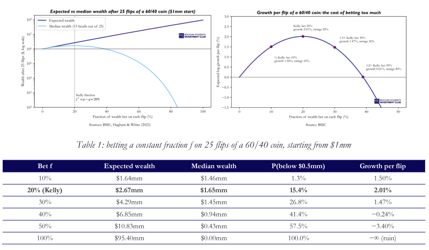
This keeps increasing with f, so an investor who maximizes expected wealth should bet everything on every flip. With f=100% expected wealth is 1.22595 times the initial $1mm, about $95mm, yet the investor loses everything at the first tail, which happens with probability 1-0.625=99.9997%. The expectation is huge only because of the 0.0003% chance of 25 heads in a row: the mean is pulled up by a handful of extremely lucky paths that almost nobody will live.
A better guide is the median outcome, the result that half of the investors beat and half do not. Here it is easy to find: final wealth only depends on the number of heads H and increases with it, and the median number of heads in 25 flips of the 60/40 coin is 15 (which is also the most likely number). Median wealth is therefore
Wmedian=W0 (1+f)15 (1-f)10
With f=20% this is 1.2150.810=1.65, i.e. $1.65mm, while with f=50% it is 1.5150.510=0.43, i.e. $0.43mm, less than we started with, even though every bet had a 60% chance of winning. Figure 1 (left) plots both quantities: expected wealth rises forever, median wealth has a clear peak at 20%. The sizing rule we are looking for should maximize median wealth, not expected wealth.
The Kelly criterion: maximizing growth
Kelly (1956) [1] made this idea precise. If we write final wealth as WT=W0 egT, then g is the growth rate per bet. With H heads out of T flips,
g=1TlnWTW0=HTln(1+f)+T-HTln(1-f)
As the number of flips grows, the share of heads H/T gets closer and closer to p (law of large numbers), so the growth rate converges to
g(f)=pln(1+f)+qln(1-f)
This is also the growth rate of the median investor, who gets about pT heads: median wealth is approximately W0 eg(f)T. Maximizing g(f) is therefore the same as maximizing median wealth, and over many bets the fraction with the highest g(f) ends up with the most money. To find it, we set the derivative to zero, using ddfln(1+f)=11+f and ddfln(1-f)=-11-f:
p1+f–q1-f=0 p(1-f)=q(1+f) p-q=f(p+q) f*=p-q
since p+q=1. For the 60/40 coin the Kelly bet is f*=0.6-0.4=20% of wealth, which grows wealth by g=0.6ln1.2+0.4ln0.8=0.109-0.089=2.0% per flip: after 100 flips the median player has multiplied wealth by e1000.027.5.
The shape of g(f) is what matters most for our message. For small bets we can use ln(1+y)≈y-y2/2 (for instance ln1.05=0.0488 against 0.05-0.00125=0.0488), which gives
g(f)≈pf-f22+q-f-f22=(p-q) f-12f2
a parabola with its top at f*=p-q and zeros at f=0 and f=2(p-q). Two consequences follow. First, the parabola is symmetric: betting 10% or 30% on the 60/40 coin gives almost the same growth (1.50% and 1.47% per flip), but the 30% bet makes wealth swing three times as much (the standard deviation of the log change in wealth is 30% per flip against 10%). Second, at about twice Kelly the growth rate is zero (exactly at 39% for this coin) and beyond it negative: median wealth then shrinks to zero even though every single bet has a positive expected value. Figure 1 (right) shows the exact curve. Betting less than Kelly costs a little growth and reduces risk; betting the same amount more than Kelly costs the same growth but adds risk. This asymmetry in risk is the first hint that Kelly is a ceiling.
Most bets are not even-money coins. In general, suppose that for every $1 bet we win rw with probability p and lose rl with probability q=1-p, where rl does not need to be 1: a trade with a stop-loss at -10%, for instance, has rl=0.1. Betting a fraction f of wealth, a win multiplies wealth by 1+frw and a loss by 1-frl, so by the same argument as for the coin
g(f)=pln(1+frw)+qln(1-frl)
Setting the derivative to zero and solving step by step (Paleologo [3], Example 13.3),
p rw1+frw=q rl1-frl p rw(1-frl)=q rl(1+frw) p rw-q rl=f rwrl(p+q)
and since p+q=1,
f*=p rw-q rlrw rl=prl–qrw
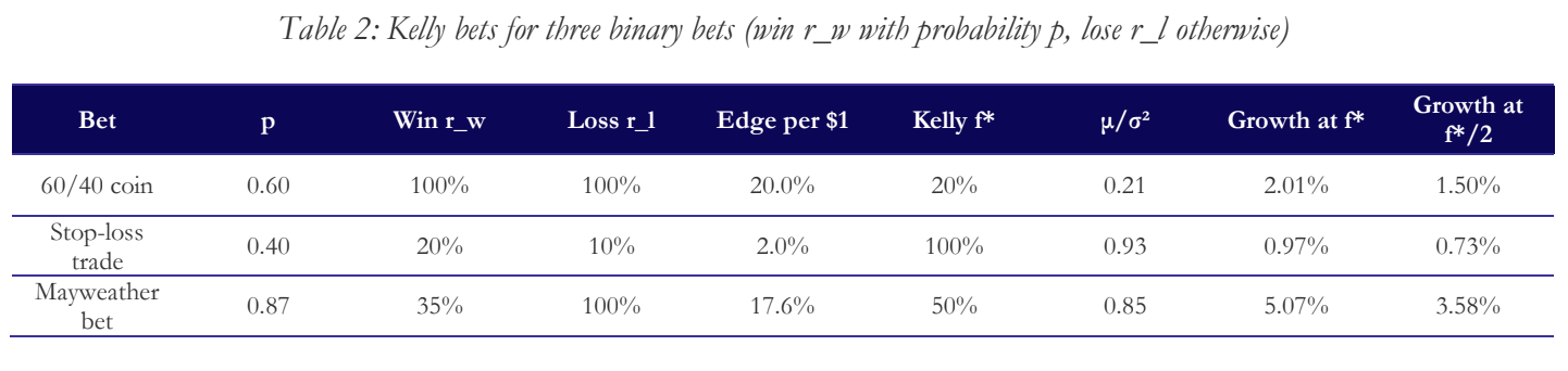
The numerator p rw-q rl is the expected gain per $1, the edge: if it is zero or negative the Kelly bet is zero. The coin is the special case rw=rl=1, which gives back f*=p-q. Take a trade that gains 20% with probability 40% and loses 10% (its stop-loss) with probability 60%. The edge is 0.40.2-0.60.1=2% per $1 and the Kelly bet is f*=0.4/0.1-0.6/0.2=4-3=100% of wealth, which grows wealth by 0.4ln1.2+0.6ln0.9=0.97% per trade. A bet of 100% is not reckless here, because the worst case costs only 10% of wealth; Kelly bets more when the possible loss is smaller. The same parabola appears: half Kelly (50%) grows 0.73% per trade, 1.5 times Kelly 0.74%, and at about twice Kelly (204%) growth is zero.
When the loss is the whole stake (rl=1) and the win is b per $1, the formula becomes f*=p-q/b, the edge pb-q divided by the odds b. A real example from [2] is the 2017 boxing match between Floyd Mayweather and Conor McGregor. Betting markets gave Mayweather a 74% chance of winning, so at the market’s odds a $1 bet on him paid b=0.26/0.74=0.35. A professional gambler put the true probability at 87%. Kelly then says to bet f*=0.87-0.13/0.35=0.50, half of one’s wealth, on a bet that adds only 18% to wealth if it wins, a size most people would find absurd.
On the theoretical side, Breiman (1961) [5] showed that for independent bets the Kelly strategy ends up, with probability one, with infinitely more wealth than any strategy with a different growth rate. This is why Kelly is so often presented as the optimal rule. What the result does not say is how bumpy the ride is, or what happens when p is not known.
From coins to markets
To move from bets to assets, it helps to rewrite the result in terms of the mean and the variance 2 of the return of the bet. For the coin, a $1 bet pays +1 or -1, so =p-q=0.2 and 2=E[r2]-2=1-0.22=0.96, and /2=0.21, almost exactly the Kelly bet of 0.20. For the stop-loss trade, =2% and 2=pq (rw+rl)2=0.40.60.32=0.0216, so /2=0.93 against the exact 1.00. In both cases the Kelly bet is close to the mean of the bet divided by its variance, and this is the form that carries over to markets. The approximation is poor only for very lopsided bets: for the Mayweather bet /2=0.85 against the exact 0.50 (Table 2), a first sign that mean and variance are not the whole story.
Consider an asset whose excess return r (the return above the risk-free rate) has mean and standard deviation , and suppose we invest a fraction x of wealth in it and keep the rest in cash (x>1 means borrowing to invest more than our wealth). Over one period wealth is multiplied by 1+xr on top of the risk-free return, so the growth rate is g(x)=E[ln(1+xr)]. Using again ln(1+y)≈y-y2/2 with y=xr, and E[r2]=2+2,
g(x)≈x E[r]-12x2E[r2]=xμ-12x2(2+2)≈xμ-12x22
where the last step drops 2, which is tiny compared with 2 over short periods (a daily mean of 0.03% against a daily volatility of 1%). The formula is exact if the portfolio is rebalanced continuously (Paleologo [3], Example 13.4). Setting the derivative -x2 to zero gives the Kelly allocation, and substituting it back gives the growth it achieves:
x*=2, g(x*)=22–1222=122=SR22
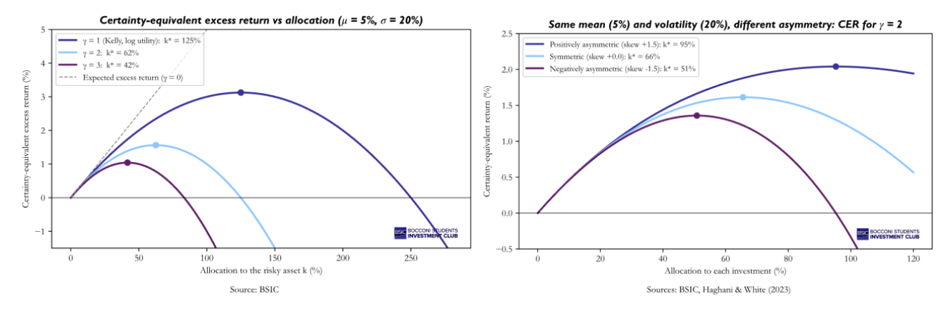
where SR=/ is the Sharpe ratio. Take the stock market with =5% and =20% per year, the base case in [2]. Kelly says x*=0.05/0.22=0.05/0.04=125%, i.e. borrow 25% of wealth to buy more stocks, for a median growth of 0.252/2=3.1% per year above the risk-free rate. Holding exactly 100% in stocks gives g(1)=0.05-120.04=3.0% per year. Going from 100% to 125% adds only 0.1% of growth per year and 25% more risk, while 250%, twice Kelly, gives g(2.5)=0.125-126.250.04=0. Near the top the curve is very flat. Note also that at full Kelly the volatility of the portfolio is x*=/, exactly the Sharpe ratio: 1.2520%=25% here.
Adding risk aversion: the Merton share
Maximizing growth ignores how much the investor dislikes risk. Haghani and White [2] handle this with the certainty-equivalent return (CER): the risk-free return that the investor would accept in place of the risky bet. For an investor with constant relative risk aversion (the standard utility U(W)=(W1--1)/(1-)) and normally distributed returns, the CER is the expected return minus a price of risk equal to /2 times the variance. With a fraction k in the asset the expected excess return is kμ and the variance is k22, so
CER(k)=rf+kμ-12k22 μ-γk2=0 k*=2=x*
where rf is the risk-free rate. This is the Merton share (Merton, 1969 [6]). For =1 the utility is lnW and CER(k)-rf is the same expression as the growth rate g(x) above, so the Kelly bettor is simply an investor with =1. An investor with =2, the base case used in [2], bets half of Kelly: 62.5% in stocks in the example above. For the Mayweather fight, the same calculation with =2 gives a bet of 28% of wealth instead of 50%.
The formula also quantifies how forgiving underbetting is. Writing the bet as a multiple of the optimum, k=k*, and substituting,
CER-rf=22–122222=–22SR2
At the optimum (=1) this is 12SR2/; betting half the optimum (=12) gives 38SR2/, three quarters of the best result, while betting twice the optimum (=2) gives zero, as if we had not invested at all (Figure 2, left). With =5%, =20% and =2: investing the optimal 62.5% is worth 1.56% per year above the risk-free rate, investing 31% is still worth 1.17%, and investing 125% is worth nothing.
Mean and variance are not the whole story, though. Haghani and White compare three bets with the same mean (5%) and volatility (20%): one that wins 45% with probability 20% and loses 5% otherwise (positive skew), a symmetric one, and one that wins 15% with probability 80% and loses 35% otherwise (negative skew). The Merton share puts 62.5% in each. Maximizing the exact expected utility with =2 instead gives 95%, 66% and 51%, and the positively skewed bet is worth about 50% more in CER (Figure 2, right). A mean-variance rule therefore oversizes bets that win small most of the time and occasionally lose big.
Why Kelly is a ceiling (1): drawdowns
Fractional Kelly means betting a constant fraction c of the Kelly allocation, x=c μ/2. Substituting into g(x)=xμ-12x22 gives the growth and the volatility of the strategy:
g(c)=c22–12c222=c-c22SR2, volatility=xσ=c SR
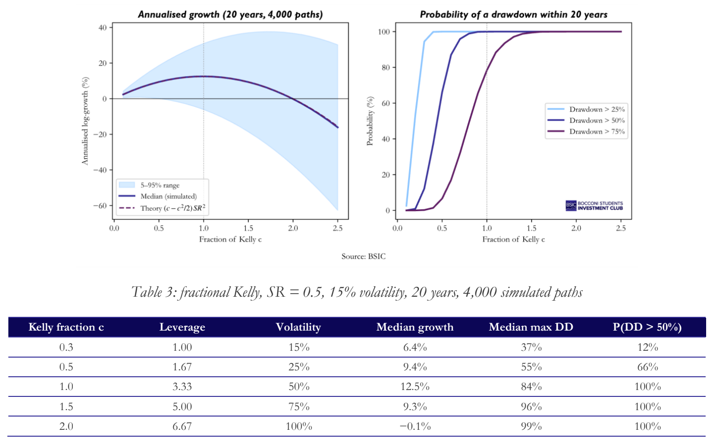
With half Kelly (c=0.5) we keep 75% of the maximum growth with half the volatility. With 1.5 times Kelly we also get 75% of the growth, but with three times the volatility of half Kelly. For a strategy with SR=0.5: full Kelly grows 0.52/2=12.5% per year with 50% volatility, half Kelly (0.5-0.125)×0.25=9.4% with 25% volatility, and 1.5 times Kelly the same 9.4% with 75% volatility. Volatility translates into drawdowns, the loss from the highest wealth reached so far. Back to the 25-flip example, the downside is very different: after 25 flips, the chance of ending with less than half the starting wealth is 15% when betting 20% (Kelly) and 1.3% when betting 10% (half Kelly).
To see this on a longer horizon, we simulated 4,000 paths of 20 years of daily returns for a strategy with a Sharpe ratio of 0.5 and a volatility of 15%, for which Kelly means a leverage of 0.075/0.152=3.3. At full Kelly the growth is 12.5% per year, but the median maximum drawdown is 84% and virtually every path loses more than half its value at some point. At half Kelly growth falls to 9.4%, the median maximum drawdown to 55% and the chance of losing half the capital to 66%; at 30% of Kelly these become 6.4%, 37% and 12% (Figure 3). No fund survives an 84% drawdown, and few investors would sit through one.
Why Kelly is a ceiling (2): we do not know the edge
All the formulas so far take and as known. In reality they are estimated, and the mean is very hard to estimate: the standard error of an average of N yearly returns is /N, so with 18% volatility even 100 years of data leave an uncertainty of 18%/100=1.8% on the expected return [2]. If our estimate is 5%, the true mean could reasonably be anywhere between 1.4% and 8.6%, and the Kelly leverage /2 anywhere between 0.4 and 2.7. Paleologo [3] shows that, under mild conditions, uncertainty always pushes the optimal bet down; for example, an uncertainty of standard deviation on the mean or on the volatility gives x*/(2+2+2).
The effect is easy to quantify when the bet is computed from an estimate, which is what happens in practice. Suppose we estimate the mean from N years of data, =+ with E[]=0 and Var()=2/N, and bet x=c /2 (for simplicity we treat as known). Our position then depends on the estimate, while our wealth grows with the true , so g=xμ-12x22. Taking expectations, with E[]= and E[2]=2+2/N,
E[g]=c22–12c22+2/N2=c SR2–12c2SR2+1N c*=SR2SR2+1/N
The noise in the estimate adds 1/N to the penalty term, so the best fraction of the estimated Kelly bet is below one, and the harder the edge is to measure (small NSR2) the lower it is. With a Sharpe ratio of 0.42 it is 0.64 with 10 years of data, 0.84 with 30 and 0.95 with 100. This puts a number on the argument of Thorp [7] that uncertainty about the edge justifies fractional Kelly.
We tested this on the US equity market with daily data from Kenneth French’s library [9], trading from January 2000 to August 2026, a period that includes the dot-com crash (−49% for the market) and the 2008 crisis (−55%). To avoid any look-ahead bias, on each day the investor uses only data available up to the day before, starting in January 1970: 30 years of history when trading starts, long enough to estimate the mean and recent enough to reflect modern markets. The expected return is the average past excess return and leverage is c /2, rebalanced daily, with two estimates of the variance: the long-run one, from all past returns since 1970, and a recent one, an exponentially weighted average of roughly the last three months, which is what volatility-targeting strategies use [4]. For comparison, Figure 4 also shows Kelly computed with hindsight, with and measured on 2000–2026 itself (SR=0.42, leverage 2.15), which no investor could have known in 2000.
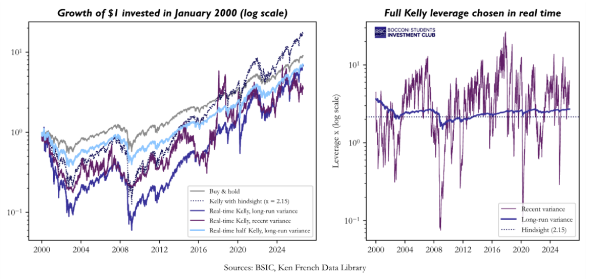
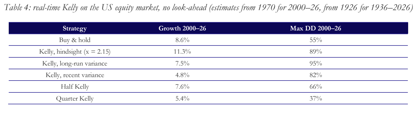
Buy-and-hold grew 8.6% per year with a maximum drawdown of 55%. In January 2000 the 30 years of data since 1970 gave =7.2% and =14.0%, so real-time full Kelly started with a leverage of 0.072/0.1423.7, just before the dot-com crash. It ended up growing 7.5% per year, less than simply holding the market, and on the way the $1 invested in January 2000 was worth $0.06 in March 2009, a 95% drawdown from its March 2000 peak. Even Kelly with hindsight, 11.3% per year, went through an 89% drawdown. With the recent variance, leverage reached 27 in the calm market of November 2017, when recent volatility was 5%, and was still 15 on 10 October 2018, when a 3.3% fall of the market cost 49% of capital in a single day. Half Kelly grew 7.6% per year, slightly more than full Kelly, with a maximum drawdown of 66% instead of 95%, and quarter Kelly 5.4% with 37%. The mistake was not in the mean, which was estimated at 7.2% against 8.2% realized over 2000–2026, but in the volatility: 14% estimated against 19.5% realized, so Kelly levered 3.7 times instead of 2.15. This is the flat top of the growth curve combined with estimation error: halving the bet cost nothing in growth and removed a large part of the risk. One should not read too much into the growth numbers, which depend on the period: running the same test from 1936, with estimates from 1926, real-time Kelly beat buy-and-hold (15.0% against 10.6% per year), but again with a 95% drawdown, while half Kelly matched buy-and-hold with 63%. The drawdown result holds in both periods; the growth result does not. The numbers are also flattering for Kelly, since we assumed borrowing at the T-bill rate without costs.
Controlling drawdowns directly: the Grossman–Zhou rule
Fractional Kelly reduces drawdowns only on average and only if the parameters are right. Grossman and Zhou (1993) [8] take a different route: maximize growth subject to never losing more than a fraction D of the high-water mark, the highest wealth reached so far. If dt is the current loss from the high-water mark, the optimal fraction invested is
ft=21-1-D1-dt
A numerical example shows how it works. With a 30% limit (D=0.3), at the high-water mark (dt=0) we invest 1-0.7=0.3 times the Kelly bet; after a 10% loss the multiplier falls to 1-0.7/0.9=0.22, after a 20% loss to 1-0.7/0.8=0.125, and at a 30% loss to zero. The bet is cut as losses accumulate, like a gradual stop-loss, and the limit can never be breached if the portfolio is rebalanced continuously.
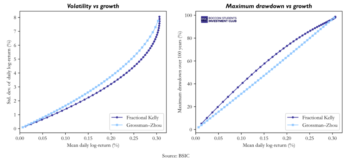
We replicated the comparison in Paleologo [3]: 100 years of simulated daily returns with a mean of 0.08% and a volatility of 1%, running both rules for all values of their parameters on the same path. Fractional Kelly has lower volatility for a given growth, but Grossman–Zhou has a lower maximum drawdown for almost any level of growth (Figure 5). With a 30% limit, it earns 0.095% per day against 0.075% for the fractional Kelly strategy with the same realized drawdown, and its limit does not depend on knowing the true parameters. The costs are a lower Sharpe ratio (1.08 against 1.24 in our simulation with D=25%), since changing exposure over time is inefficient when returns are independent, and long periods with almost no exposure after a deep drawdown.
Application: a poker bot
In a poker bot, Kelly should not be read as an instruction to bet a fixed percentage of the stack whenever the bot has an edge. Poker bet sizing has two layers. The first is strategic: a bet of one third pot, two thirds pot or an overbet changes the opponent’s calling range, folding frequency and future decisions. The second is bankroll management: how much of the bot’s capital should be exposed to a line whose edge is only estimated. Kelly belongs mainly to the second layer. The bot should first choose candidate actions from poker logic, then use fractional Kelly and drawdown limits to decide whether the risk is acceptable.
For each decision the bot can score a small menu of legal sizes, for example fold, call, 33% pot, 66% pot, pot and all in. For each size it estimates three quantities: equity when called, the probability the opponent folds, and the distribution of future gains and losses if the hand continues. A simple river bet is close to a binary bet. If the bot risks C chips to win the current pot P, and its model says the bet succeeds with probability p after combining folds and showdown wins, the edge is roughly pP – (1-p)C. The Kelly idea says the bot should increase size only while this edge grows faster than the risk. A larger bet may have more fold equity, but if it also gets called by a stronger range, its growth rate can fall even when its expected chip value looks positive.
The practical rule is therefore to separate table EV from bankroll EV. The solver or hand model can rank sizes by expected chips, but the execution module caps the amount risked as a fraction of bankroll. For a cash-game bot this bankroll is not the stack on the table but the total capital allocated to the strategy. If one buy-in is only 1% of bankroll, then even an all-in decision cannot lose more than 1% of bankroll; if the bot sits with 20% of bankroll, the same all-in is far too large. This is the poker version of the stop-loss example above: the right fraction depends on the maximum loss, not only on the chance of winning the hand.
Because the edge estimate is noisy, the bot should normally play below the raw Kelly size. Equity estimates depend on opponent ranges, rake, position, stack depth and card removal, and the model will be wrong most often in the rare large pots that dominate variance. A useful implementation is to compute a Kelly cap for the candidate line, multiply it by a conservative fraction such as 0.25 or 0.50, and then apply hard limits: maximum buy-ins per table, maximum daily loss, and a drawdown rule that reduces stake size after losses. When the bankroll is 10% below its high-water mark, the bot can cut the Kelly fraction; near the drawdown limit it can stop opening new tables or play only the lowest-volatility lines.
Testing should start away from real money. The first test is a hand-level simulation: feed the bot millions of generated spots or historical hands, hide the villain’s cards until showdown, and record EV by action size. The second test is bankroll Monte Carlo. Resample complete sessions, including rake and realistic table limits, and compare fixed sizing, half Kelly, quarter Kelly and a drawdown-controlled rule. The output should not be only bb/100. It should include volatility, worst drawdown, probability of losing 25% or 50% of bankroll, time spent under the high-water mark and sensitivity to model error.
The most important stress test is deliberate overconfidence. If the bot thinks it has 55% equity in a spot where the true number is 51%, full Kelly will oversize the bet and the damage will appear only after many hands. A good test perturbs the estimated fold frequencies and equities before sizing the bet, then checks whether the strategy still survives. The final bot should pass three tests before deployment: it wins in chip EV, it grows bankroll under conservative fractional Kelly, and it stays within a drawdown limit under pessimistic assumptions. If those three tests disagree, the sizing module should choose survival over theoretical growth. In future articles, we will likely develop and test bots capable of reading hands, tracking as many relevant inputs as possible, and optimizing bet size as efficiently as possible given the chosen playing strategy.
Conclusion
The Kelly criterion answers a real question: the fraction of wealth that maximizes long-run growth is p-q for an even-money bet and /2 for an asset, and an investor who bets far more than that will lose money even with an edge. But growth near the Kelly bet is flat, so betting less costs little, while betting more costs the same growth with more risk. Add drawdowns that few investors can bear, an edge that can only be estimated with a large error, and returns that are not normal, and the conclusion is that Kelly is a ceiling, not a target.
In practice this suggests a simple recipe: estimate the Kelly bet, bet a fraction of it, lower when the edge is uncertain (half Kelly is a common choice, and SR2/(SR2+1/N) gives an idea of how much to cut), and add an explicit drawdown rule such as Grossman–Zhou if large losses are not acceptable. The poker bot example makes the same recipe concrete: estimate the edge of each candidate line, cap the money at risk with fractional Kelly, and reduce exposure when drawdowns or model uncertainty rise.
References
- Kelly, John L. (1956), A New Interpretation of Information Rate, Bell System Technical Journal.
- Haghani, Victor; White, James (2023), The Missing Billionaires: A Guide to Better Financial Decisions, Wiley.
- Paleologo, Giuseppe A. (2025), The Elements of Quantitative Investing, Wiley.
- Kolanovic, Marko; Wei, Zhen (2013), Systematic Strategies Across Asset Classes: Risk Factor Approach to Investing and Portfolio Management, J.P. Morgan.
- Breiman, Leo (1961), Optimal Gambling Systems for Favorable Games, Proceedings of the Fourth Berkeley Symposium on Mathematical Statistics and Probability.
- Merton, Robert C. (1969), Lifetime Portfolio Selection under Uncertainty: The Continuous-Time Case, Review of Economics and Statistics.
- Thorp, Edward O. (2006), The Kelly Criterion in Blackjack, Sports Betting and the Stock Market, Handbook of Asset and Liability Management.
- Grossman, Sanford J.; Zhou, Zhongquan (1993), Optimal Investment Strategies for Controlling Drawdowns, Mathematical Finance.
- French, Kenneth R., Data Library: Fama/French 3 Factors (Daily), Tuck School of Business.


0 Comments