Is Cheap a Trade?: Mexico’s Mispriced Duration or a New Term-Premium Regime?

Download PDF

Introduction

Mexico’s government-bond curve presents an unusually steep front-to-intermediate structure, but the distinction between a steep macro curve and a locally cheap five-year bond has become increasingly important. At research inception, Banco de México’s overnight target stood at 6.50%, while the S&P benchmark curve placed the 1Y at 6.81%, the 3Y at 7.38%, the 5Y at 8.71% and the 10Y at 9.52%. The corresponding 1s5s spread was about 190bp and near the 99th percentile of the cleaned 2016-2026 monthly sample. These observations motivated the original receive-5Y/pay-front-end hypothesis.

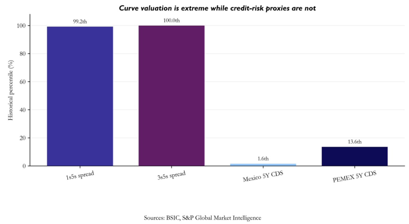
Headline inflation fell to 3.26% year-on-year in August 2026, but core inflation remained 3.88%, and private-sector specialists still expect inflation over the following twelve months at roughly 4.2%. Meanwhile, credit markets tell a different story: the cost of insuring Mexico and PEMEX debt against defined credit events remains unusually low relative to the past decade. The curve is therefore pricing substantial medium-term compensation without corresponding extreme credit-event stress.

This article tests whether that compensation is a tradable mispricing. We explain the bond mathematics behind the curve, forward rates, DV01-neutral relative-value trades, carry and roll, before decomposing the curve and testing five competing explanations for its steepness. Rather than treat a mechanical backtest as proof of alpha, the final section asks what distribution of 1M, 3M and 6M outcomes historically followed comparable high-curve states. 

The central distinction that emerges is that an extreme slope is not equivalent to an equally large five-year mispricing. Bond-specific models initially identified local 5Y cheapness of roughly 8-25bp, materially smaller than the approximately 190bp 1s5s slope. Moreover, the raw macro spread does not exhibit robust stationarity, whereas some local relative-value residuals show considerably stronger mean-reversion evidence. The analysis therefore separates three questions that are often conflated: whether the curve is historically extreme, whether the 5Y is locally cheap relative to surrounding maturities, and whether either condition predicts profitable convergence.

Why This Matters Now

The timing is significant because Mexico’s 1s5s curve remains near the 99th percentile of the cleaned 2016–2026 sample, while Banxico’s 24 September decision left the overnight target unchanged at 6.50%. The hold preserved the near-term policy anchor, but Banxico still described inflation risks as tilted upward: core inflation was 3.79% in the first half of September, headline inflation 3.42%, and convergence to the 3% target is expected only in Q4 2027. The curve therefore still embeds substantial compensation beyond the front end despite no immediate policy tightening.

That premium is consistent with broader risk conditions. Banxico noted higher US yields, a stronger dollar, firmer commodity prices and higher Mexican government yields across most maturities, while domestic fiscal concerns remain live following S&P’s negative outlook and Moody’s Baa3/stable rating. The question is therefore whether the steep curve reflects temporary overcompensation that can converge, or a more persistent term-premium regime driven by inflation, fiscal, global-duration and supply risks.

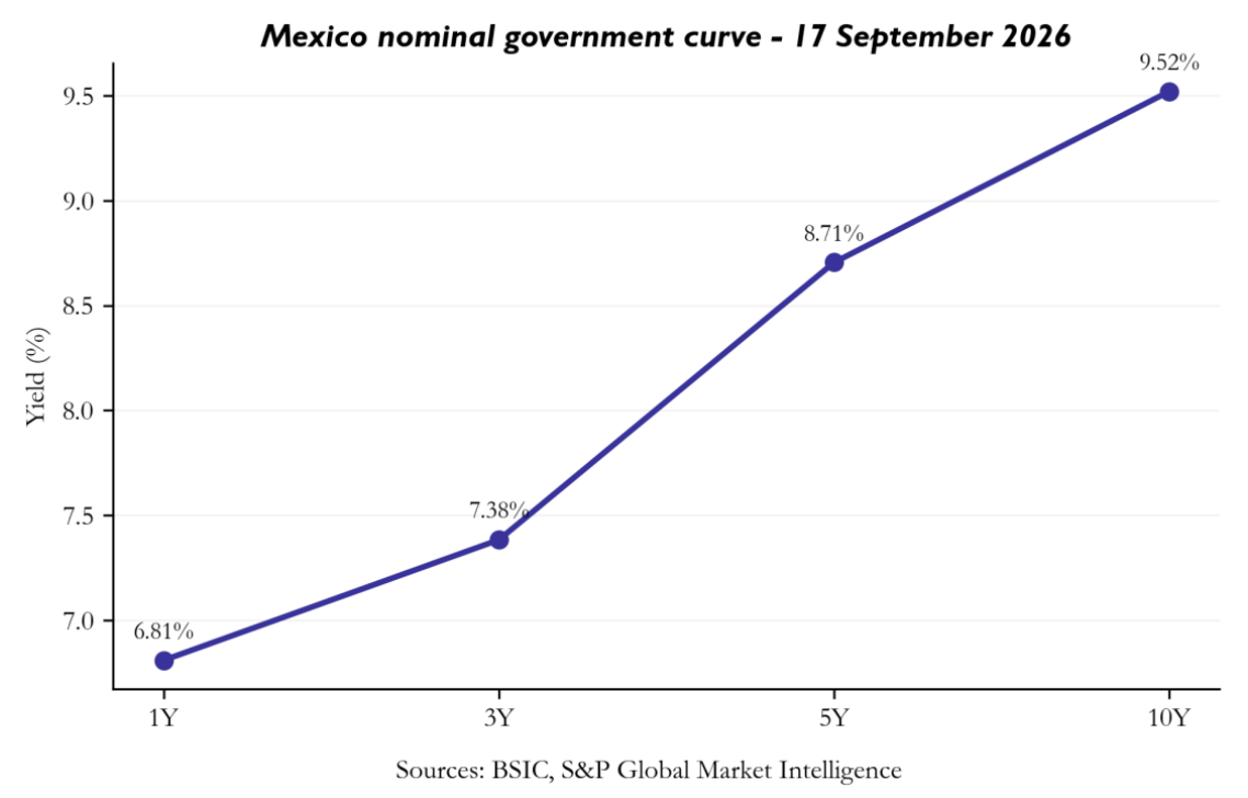
The Post-Meeting Curve

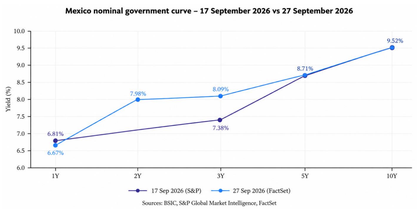
The 27 September curve remains steep, but its shape changes the interpretation of the original signal. The 1Y, 2Y, 3Y and 5Y benchmarks stand at 6.67%, 7.98%, 8.09% and 8.71%, respectively, leaving 1s5s at roughly 204bp. However, around 131bp, approximately 64%, of that slope now occurs between 1Y and 2Y. The 2s5s and 3s5s spreads are much smaller at roughly 73bp and 63bp. The extreme 1s5s reading therefore increasingly reflects the shape of the front end rather than an isolated cheapening of the 5Y point.

The 3Y is particularly important for the thesis. It stands at 8.09% on 27 September versus 7.38% on 17 September, while the quoted 5Y and 10Y levels are essentially unchanged. Because the two snapshots use different benchmark vendors, the difference is interpreted cross-sectionally rather than as a measured market return. Cross-sectionally, however, the higher current 3Y substantially compresses the local 3s5s slope and weakens the case that the 5Y itself is the source of the curve’s extremeness. The post-meeting evidence therefore shifts the thesis toward a broader front-end and term-premium dislocation rather than a simple 5Y-specific mispricing.

Why the Mexican Curve Looks Like a Trade

The dislocation can be summarized simply: medium-term compensation remains elevated relative to the current policy rate and front end even though Banxico is no longer in the high double-digit policy-rate regime. The choice of 1s5s rather than 2s5s is dictated by data quality. The supplied S&P rate profile contains a consistent observed 1Y and 3Y history but not a consistent 2Y benchmark history. The initial research package interpolated a 2Y point between 1Y and 3Y for diagnostics; that interpolation is unsuitable for an executable historical trade analysis. 

The Instruments Behind the Trade

The phrase “Mexican rates” covers several instruments with different cash flows and risk exposures. The front end of the local government market is represented principally by CETES, zero-coupon federal Treasury certificates issued at a discount and redeemed at par. Their price-yield relationship is especially transparent: the investor’s return comes from the difference between purchase price and face value. Short CETES therefore provide a natural reference for near-term monetary-policy expectations and funding conditions.

Further out the curve, the relevant nominal instruments are fixed-rate Bonos M. A five-year Bono consequently contains a sequence of cash flows whose value depends on the entire discount curve. Benchmark-yield services summarize that pricing into a quoted yield, but the security itself is a coupon-bearing bond. This is why treating a benchmark 5Y yield as a zero rate is an approximation when deriving forwards.

Mexico sovereign CDS and PEMEX CDS measure different credit risks. Mexico sovereign CDS is an insurance-like derivative on a defined credit event of the sovereign: the protection buyer pays a periodic premium, quoted in basis points on a reference notional, and the seller compensates the buyer if a qualifying credit event occurs. PEMEX CDS works the same way but references Petroleos Mexicanos, the state-owned oil company. PEMEX matters to the sovereign curve because government support can turn weakness at the company into a contingent fiscal liability, but PEMEX debt is not identical to sovereign debt and its CDS can move independently. A 78.81bp Mexico five-year CDS quote corresponds, before standard contractual adjustments, to roughly 0.7881% of reference notional per year, or about $78,810 on $10m. 

Finally, the foreign investor faces MXN currency exposure. A peso-denominated Bono can outperform in local terms and still lose money in dollars or euros if the peso depreciates sufficiently. A pure rates desk can isolate the local curve through swaps or FX hedging; an unhedged global investor cannot. The probability and P&L analysis in this article therefore measures local rates alpha in matched-DV01 terms and treats FX as a risk variable.

Bond Mathematics: From Yield to Relative-Value P&L

A fixed-rate government bond is a stream of promised cash flows written as the discounted value of coupons and principal:

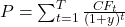
When a single yield-to-maturity is used, the same discount rate is imposed on all cash flows. In a more rigorous term-structure framework, each cash flow is discounted using the zero-rate corresponding to its maturity. That distinction matters when we construct forward rates, because benchmark bond yields are not themselves zero-coupon yields. Forward rates are constructed from zero rates because they compare investment over precise future intervals. Treating a coupon-bond benchmark yield as if it were a zero rate is therefore an approximation: it can overstate or understate the implied forward when the curve is steep or curved. This is the measurement problem that motivates the Nelson-Siegel robustness check below.

For small yield changes, modified duration gives the first-order price sensitivity:

DV01 translates that sensitivity into money. It is approximately the change in the bond’s price for a one-basis-point change in yield:

For a curve trade, matching notionals is insufficient. A $10m five-year bond position carries much more interest-rate sensitivity than a $10m one-year position. To remove the first-order parallel shift exposure, the two legs must satisfy:

where N_1 and N_5 are the notionals of the front-end and five-year legs. A receive-5Y/pay-1Y flattener then has approximately zero net DV01 to a parallel move, while retaining exposure to the change in the slope:

If both legs have $10k of DV01, a 1bp fall in the 1s5s spread produces about $10k of first-order P&L before carry, roll, convexity and transaction costs. More generally:

Carry is the income earned from holding the position if the curve is unchanged. Roll-down is the mark-to-market effect of a bond aging along an unchanged yield curve. In an upward-sloping segment, a bond can roll toward a lower-yielding maturity and gain price; in an inverted segment, the opposite can occur. Institutional rates trading therefore evaluates a curve trade using expected convergence plus carry and roll, not a z-score alone.

Convexity adds a second-order term:

For relatively modest yield changes, DV01 provides a useful first-order approximation. For large stress scenarios, convexity should be included. 

Forward Rates Are Not Policy Forecasts

Step 1 – What a forward rate actually means

A spot or zero-coupon yield answers a simple question: what annualized return can be locked in today from now until one particular maturity. Suppose an investor wants money invested from today to year five. Strategy A locks the five-year zero rate today. Strategy B locks a three-year zero rate today and, at year three, reinvests for the final two years at the forward rate implied today. No-arbitrage requires the two compounded payoffs to match:

Solving for the two-year rate beginning in year three gives:

Using the 17 September S&P benchmark points as approximate zero rates, z3 = 7.383% and z5 = 8.705%, which gives an indicative 3Y-to-5Y forward of about 10.72%. The same arithmetic using the 1Y and 5Y points gives about 9.18% for the average rate between years one and five. Economically, the curve is saying that an investor who gives up the shorter maturity needs much more compensation to hold exposure farther into the future.

Step 2 – Why that is not a Banxico forecast

The crucial interpretation is that a sovereign forward rate contains more than expected future policy rates. Investors also require compensation for uncertainty about inflation, real rates, fiscal policy, liquidity, duration supply and how those risks behave in bad states of the world. A useful conceptual decomposition of an n-year yield is:

The first term is the average expected path of future short rates; TP is the term premium, a catch-all for compensation investors demand for bearing duration and state-contingent risk. 

Step 3 – Nelson-Siegel: using the whole curve instead of two points

Nelson-Siegel is used here as a cross-sectional robustness check. A raw forward constructed from two benchmark maturities can move sharply if either quote is noisy. Fitting one smooth curve to all twelve benchmark maturities from 1M to 30Y asks whether the same valuation signal survives when the inference is constrained by the broader term structure rather than one maturity pair.

For maturity τ, the fitted yield is:

The equation is easiest to read as three additive factors. β₀ is level: it shifts the whole curve and is the yield approached at very long maturities. β₁ is slope: its loading is strongest at the short end and fades toward zero, controlling the gap between short rates and the long-run level. β₂ is curvature: its loading is small at the shortest and longest maturities but largest in the intermediate sector, allowing the curve to hump or dip. Finally, λ controls how quickly the slope loading decays and therefore where the curvature effect is concentrated.

The limiting cases make the interpretation precise:

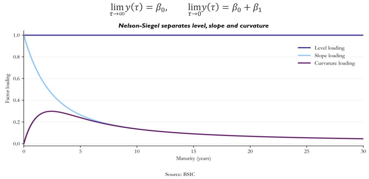
The parameters are chosen to minimize the squared distance between observed benchmark yields and the fitted curve:

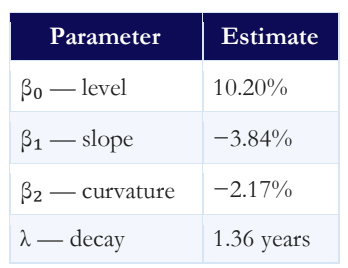
With twelve benchmark maturities and four fitted parameters, the 22 September cross-sectional RMSE is approximately 21bp. That error is economically meaningful rather than negligible: Nelson-Siegel should not be presented as the true term structure, and individual fitted points are not exact market prices, however its value is robustness, preventing one pair of raw benchmark yields from determining the conclusion.

Step 4 – What the smoothed curve changes

Using the Nelson-Siegel fitted yields as zero-rate proxies gives an indicative average 1Y-to-5Y forward of about 9.08% and a 3Y-to-5Y forward of about 9.63%. The second number is materially below the crude 10.72% two-point calculation. That is the first contribution of the model to the thesis: part of the apparent forward-rate extremeness was a measurement effect created by treating two coupon-bond benchmark yields as if they were exact zero rates.

The second contribution is economic. Smoothing does not eliminate the wedge. A 3Y-to-5Y forward near 9.6% still sits well above the roughly 6.5% Banxico path expected by private-sector forecasters. Nelson-Siegel therefore weakens the size of the valuation signal, but it does not overturn it.

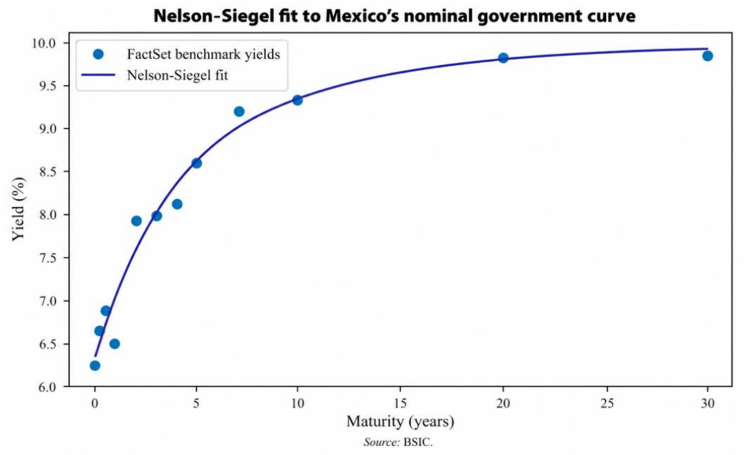
Repeating the same cross-sectional Nelson-Siegel exercise on the 27 September curve produces a fit with an RMSE of roughly 21bp and an indicative 3Y-to-5Y forward around 9.7%. The broad forward-rate wedge therefore survives the new developments.

Is the Five-Year Sector Actually Cheap?

The headline 1s5s spread answers a macro curve question: is the five-year yield unusually high relative to the front end? It does not tell us whether the five-year point itself is mispriced relative to the rest of Mexico’s curve. We therefore separate broad slope from local five-year relative value. 

How We Test Whether a Relative-Value Gap Mean-Reverts

Before using the Augmented Dickey–Fuller (ADF) test, the Kwiatkowski–Phillips–Schmidt–Shin (KPSS) test or a half-life, we need to define the economic question. Suppose a curve spread or a five-year relative-value residual looks unusually high today. That observation alone does not tell us whether it should fall. The series could be temporarily displaced from a stable long-run level, in which case mean reversion is plausible, or it could be moving through a new regime whose long-run level itself is changing. The tests below are designed to distinguish those two behaviours. 

Let x_t denote whichever object we are testing: raw 1s5s, the regression-implied 5Y residual, the leave-5Y-out Nelson-Siegel residual or the 3s5s10s fly. An AR(1) model says that today’s value depends on a constant, a fraction rho of last month’s value and a new shock:

The coefficient rho measures persistence. If 0 < rho < 1, a shock gradually loses influence: the series has a tendency to return toward a stable level. A rho close to one means that this decay is very slow. The special case rho = 1 is called a unit root:

With a unit root, there is no built-in pull back toward a fixed mean. A positive shock raises the level today and that higher level becomes the starting point for tomorrow; shocks can therefore accumulate rather than decay. Rejecting a unit root does not prove that a trade will make money, but it is evidence against this permanent-shock behaviour and in favour of a process that is more consistent with mean reversion around a stable level or deterministic component.

The ADF test formalizes that question. It rewrites the process in changes and asks whether the previous level helps predict a movement back in the opposite direction:

Here, Delta x_t is this month’s change; x_(t-1) is last month’s level; gamma is the restoring-force coefficient; the lagged Delta x terms absorb short-run momentum and serial correlation; and epsilon_t is a new unexplained shock. If x_(t-1) is unusually high and gamma is negative, the model predicts a negative subsequent change, pulling the series downward. If the level is unusually low, the same negative gamma works in the opposite direction. The ADF hypotheses are:

The ADF null hypothesis assumes there is a unit root and no statistically established restoring force. A small ADF p-value means the observed data would be difficult to reconcile with that null, so we reject the unit-root hypothesis. For example, p = 0.046 is below a 5% significance threshold and provides evidence against a unit root. 

KPSS deliberately asks the question in the opposite direction. A useful way to understand it is to split the observed series into a long-run component mu_t and a temporary stationary disturbance u_t. The long-run component is allowed to move only if it receives its own innovation eta_t:

KPSS tests whether the variance of those long-run innovations is zero:

If Var(eta_t) = 0, the long-run level is not wandering through time, so the KPSS null is stationarity. A small KPSS p-value therefore rejects stationarity; a large p-value means we do not have enough evidence to reject it. This is the reverse of ADF. Using both tests is useful precisely because their null hypotheses point in opposite directions.

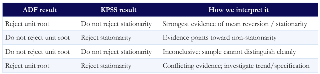
The p-value itself asks how unusual the observed test statistic would be if the null hypothesis were true. We use 5% as the conventional reference threshold, but results close to that boundary should be interpreted as evidence rather than a binary truth. In this article, the strongest mean-reversion evidence occurs when ADF rejects a unit root while KPSS does not reject stationarity.

Only after stationarity is reasonably credible does a half-life become economically meaningful. 

If there are no further shocks, the expected remaining deviation after h periods is:

Half-life asks for the horizon at which only one-half of the original deviation remains. Setting rho to that condition gives:

For intuition, if rho = 0.80 at a monthly frequency, the half-life is about 3.1 months: a 20bp deviation would be expected to shrink to roughly 10bp after about three months if the same stationary process continued to hold. If stationarity is not established, we report the mechanical AR(1) half-life only descriptively and do not use it as a trading horizon.

Test 1 – Historical curve-implied 5Y relative value benchmark

Our first bond-specific model asks where the 5Y would normally trade given the observed 1Y, 3Y and 10Y Mexican yields. We use an expanding window: at each month t, the regression is estimated on observations available through t−1, those coefficients are used to estimate the 5Y curve-implied value at t, and the sample then expands by one observation before the next estimate. This prevents future information from entering the historical curve-implied benchmark:

Here, α is the baseline level and each β is the sensitivity of the 5Y yield to one neighbouring maturity after holding the others fixed. We define the five-year residual as observed 5Y yield minus fitted 5Y yield. A positive residual therefore means the observed 5Y yield is above the surrounding-curve estimate while a negative residual means it is rich. Since every fitted value is generated using only earlier observations, the residual series is genuinely out-of-sample.

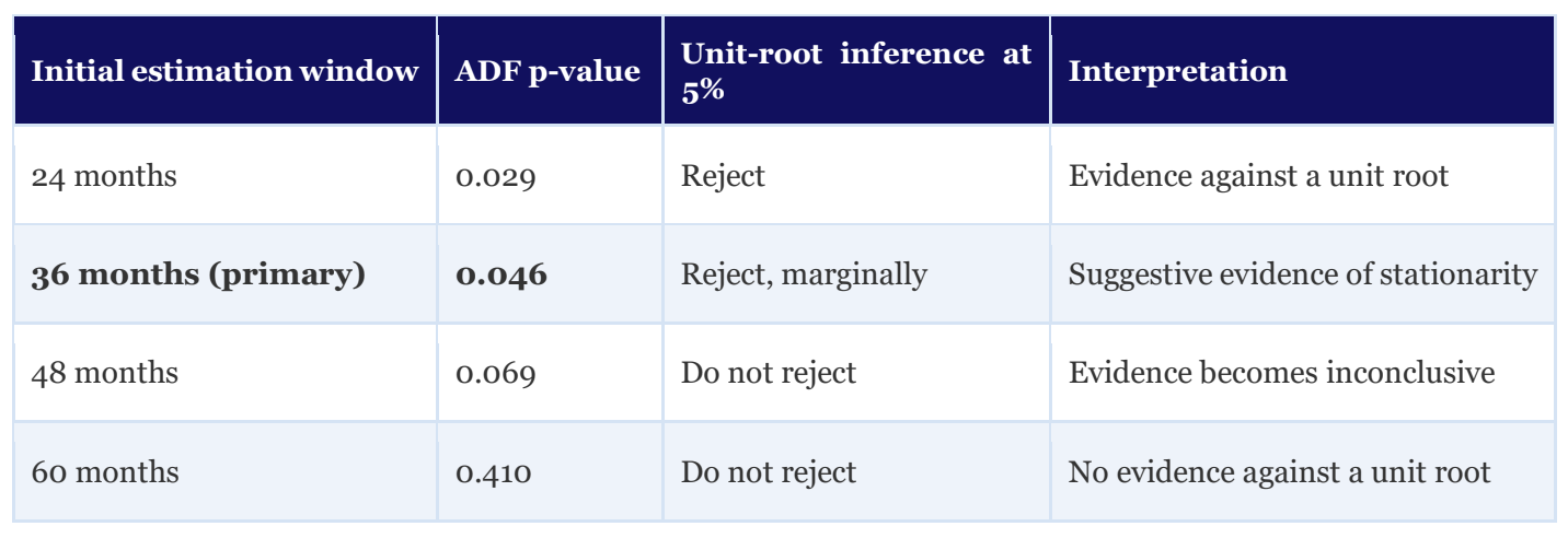
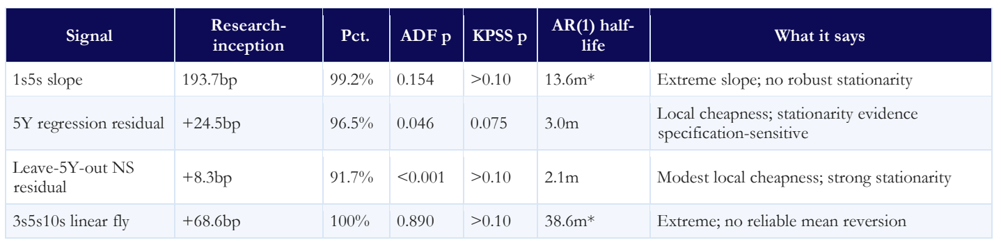
Using the 36-month initialization adopted for the primary specification, the latest research-inception residual is approximately +24.5bp, around the upper tail of its available out-of-sample history. ADF rejects a unit root only marginally at the conventional 5% threshold, while KPSS does not reject stationarity. The result is therefore suggestive rather than definitive. In particular, robustness checks show that the formal ADF inference weakens when longer initialization windows are used, so the regression residual should be treated as supporting evidence of local relative value rather than as proof of a stable convergence process.

Test 2 – Leave-the-5Y-out Nelson-Siegel residual

Using the Nelson-Siegel framework introduced above, a cleaner robustness check removes the 5Y observation entirely, fits the remaining 1Y, 3Y, 7Y, 10Y, 20Y and 30Y points each month, and asks what that smooth surrounding curve predicts at five years. The relative-value residual is:

At research inception, the residual was about +8.3bp, around the 92nd percentile of the historical sample. ADF strongly rejects a unit root (p<0.001), KPSS does not reject stationarity, and the descriptive AR(1) half-life is about two months. The result supports modest, mean-reverting local 5Y cheapness but far less than the roughly 190bp raw 1s5s slope.

Test 3 – A simple 3s5s10s curvature check

As a transparent non-parametric cross-check, we compare the observed 5Y yield with a straight-line interpolation between the 3Y and 10Y points. The five years lies two years beyond 3Y within a seven-year interval. Thus, the interpolated 5Y places 5/7 weight on the 3Y yield and 2/7 on the 10Y yield. The fly is the observed 5Y yield minus that interpolated value: a positive reading means the 5Y sits above the line joining its two wings and therefore looks cheap in yield terms. 

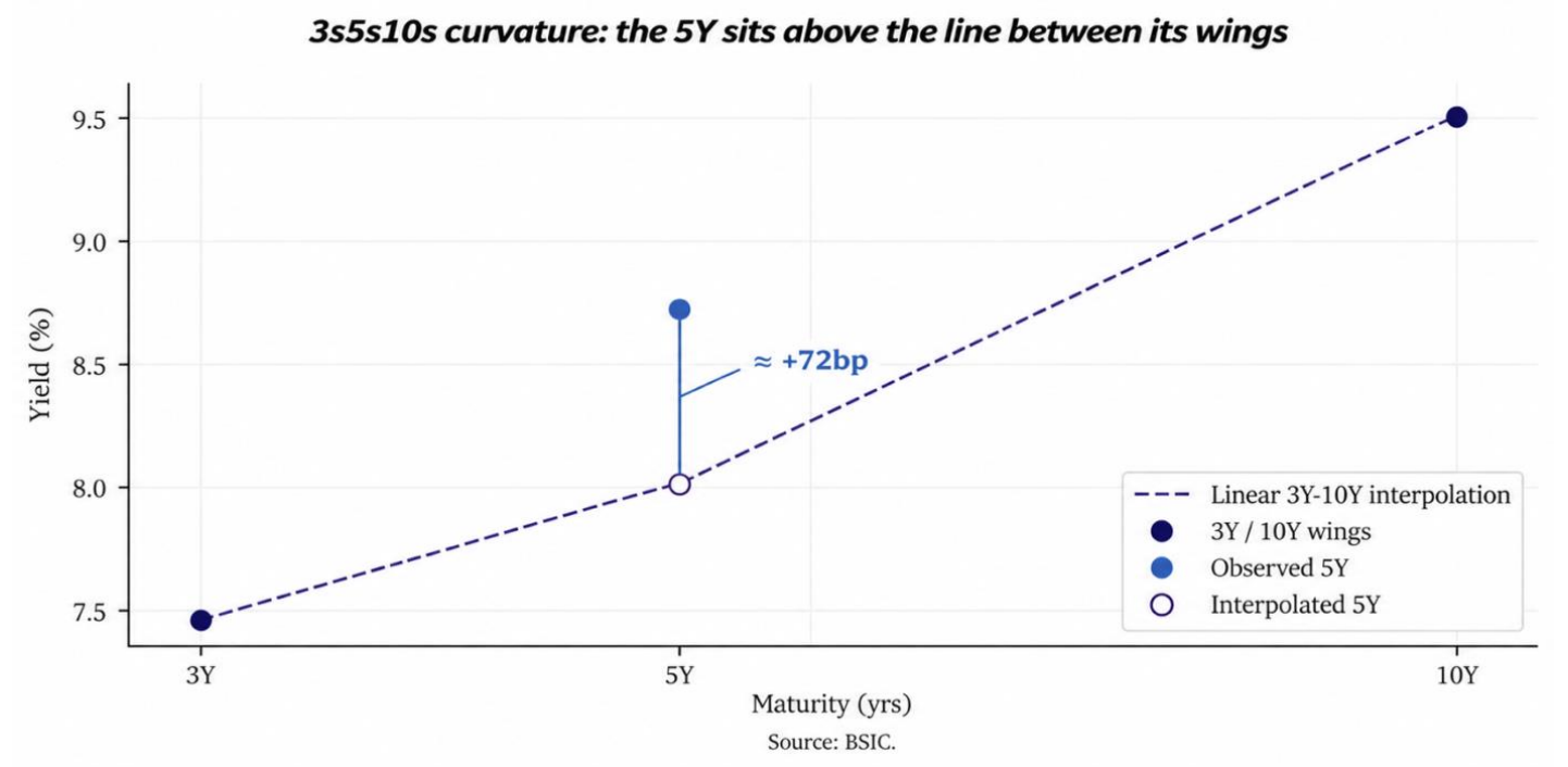
At research inception, the curvature residual was roughly +69bp and sits at the top of the sample. The statistical evidence, however, argues against treating it as a convergence trade: ADF strongly fails to reject a unit root (p=0.89), and historically high readings did not reliably narrow over the following one, three or six months. The fly is therefore useful evidence that the current curve is unusually shaped, but not evidence of a stable equilibrium around which a 3s5s10s butterfly can be expected to mean-revert. 

What the bond-specific models contribute to the thesis

Taken together, the models sharpen the original thesis. Raw 1s5s is exceptionally steep, but that spread is not robustly stationary. Bond-specific models do identify positive 5Y cheapness, and their residuals are more mean-reverting, but the estimated magnitude ranges from roughly 8bp under leave-5Y-out Nelson-Siegel to roughly 25bp under the walk-forward surrounding-curve regression. The evidence therefore does not support describing the entire 190bp slope as a five-year mispricing. It supports a narrower statement: the five-year sector contains a modest local cheapness embedded inside a much larger macro curve regime.

Does the 1s5s Flattener Itself Mean-Revert?

Applying the stationarity framework above to monthly 1s5s gives an inconclusive result. The ADF p-value is 0.154, so the unit-root null cannot be rejected at conventional levels, while KPSS also does not reject stationarity at the 10% level. The 3s5s spread is weaker still, with an ADF p-value near 0.98. The disciplined conclusion is therefore that the sample does not establish a reliable convergence process. The fitted monthly 1s5s AR(1) coefficient is about 0.95, mechanically implying a 13.6-month half-life. We do not use that number as a trading horizon because stationarity is not established. 

Structural Breaks: A Stable Mean Cannot Be Assumed

The 2016–2026 sample spans several distinct monetary and macroeconomic environments, including the pandemic, the subsequent inflation shock, Banxico’s tightening and normalization cycles, and large changes in global duration conditions. This creates an important limitation for the Augmented Dickey–Fuller (ADF) and Kwiatkowski–Phillips–Schmidt–Shin (KPSS) tests used above: a series can appear highly persistent because its underlying equilibrium has changed, rather than because it follows a genuine unit-root process. 

We therefore complement the baseline tests with the Zivot–Andrews unit-root test, which explicitly allows for one structural break. Rather than choosing the break date in advance, the procedure evaluates possible dates within the sample and selects the one providing the strongest evidence against a unit root. Its null hypothesis is that the series contains a unit root; the alternative is that it is stationary around a process whose level and/or trend changes once. 

For raw 1s5s, the procedure identifies a structural break around 2022, consistent with a period of substantial change in inflation and monetary conditions. However, even after allowing for this break, the test still fails to reject the unit-root null (p≈0.42). This reinforces the baseline ADF result (p=0.154): the available sample does not establish that shocks to the macro slope reliably decay back toward a stable equilibrium. Consequently, the mechanically estimated 13.6-month AR(1) half-life should not be interpreted as a trading or convergence horizon.

Post-Meeting Update: The Local 5Y Signal Has Changed

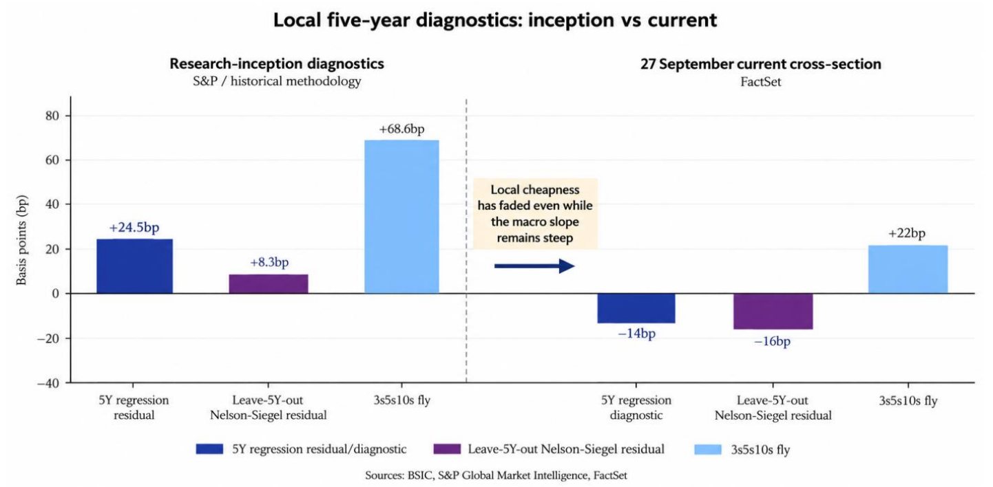
The 27 September cross-section provides an out-of-sample update to the original relative-value thesis. At research inception, all three diagnostics pointed toward local 5Y cheapness: the walk-forward regression residual was +24.5bp, the leave-5Y-out Nelson–Siegel residual +8.3bp, and the 3s5s10s fly +68.6bp. In the latest cross-section, the first two signals have reversed. The surrounding-curve regression implies a 5Y yield of roughly 8.85% against an observed 8.71%, producing a residual near −14bp, while the leave-5Y-out Nelson–Siegel fit implies approximately 8.87%, corresponding to a −16bp residual. Under the article’s sign convention, both now indicate that the 5Y is modestly rich, rather than cheap, relative to its surrounding curve.

The simple 3s5s10s fly remains positive at approximately +22bp, but has fallen substantially from the +68.6bp research-inception reading. Taken together, the diagnostics show that the original local 5Y anomaly has largely disappeared even though the broader curve remains unusually steep. This suggests the full 1s5s steepness cannot be interpreted as a five-year-specific mispricing and instead a larger share of the remaining dislocation appears to reflect the broader front-end shape and macro term premium.

Five Competing Explanations for the Steep Curve

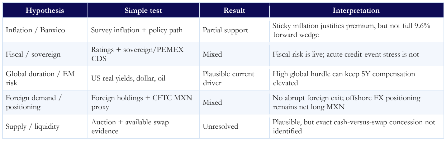
If simple mean reversion is not the answer, why is the curve so steep? We test five non-exclusive explanations with the data available rather than selecting one narrative ex ante. 

Hypothesis 1 – Incomplete inflation normalization

Inflation provides a plausible reason for Mexico’s medium-term yields to remain above the current policy rate. Nominal sovereign yields compensate investors for expected real rates, expected inflation and associated term and inflation-risk premia. In principle, part of this compensation can be observed through the difference between comparable nominal and inflation-linked yields:

The inflation data support some continued premium. August headline inflation was 3.26%, while core and services remained higher at 3.88% and 4.33%; by the first half of September, headline had risen to 3.42% while core eased to 3.79%. Banxico continues to judge inflation risks as tilted upward and expects convergence to its 3% target only in Q4 2027. Inflation normalization is therefore incomplete rather than finished.

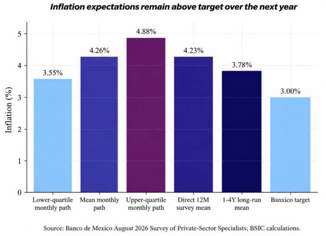
Survey expectations reinforce this picture. The August Banxico survey places the mean expected monthly inflation path at approximately 4.26%, with a wide 3.55–4.88% interquartile range, while the direct twelve-month expectation is 4.23% and the one-to-four-year mean remains around 3.78%. The latest FactSet consensus similarly places inflation around 4.1% in 2026 and 3.7% in 2027–28. Expectations therefore remain above the 3% target across both near- and medium-term measures, supporting a positive inflation-risk premium in nominal yields.

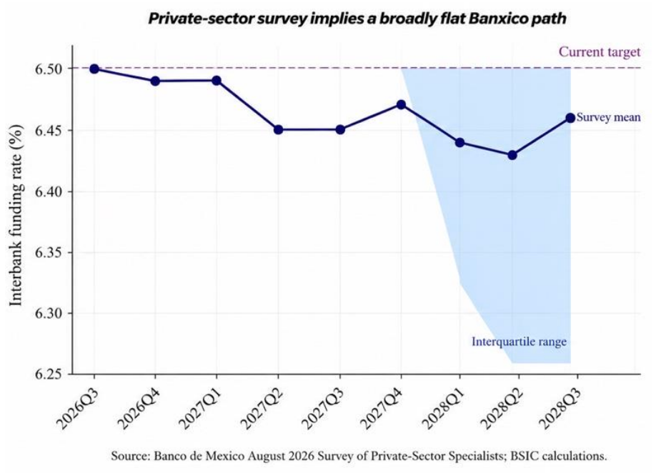
However, forecasters do not translate persistent inflation into a renewed tightening cycle. The survey-implied funding-rate path remains broadly anchored around 6.4–6.5% through 2027–28, close to the current 6.50% target that Banxico maintained on 24 September. This contrasts sharply with the curve: even after Nelson–Siegel smoothing, the indicative 3Y-to-5Y forward remains around 9.6–9.7%. The difference should not be interpreted as the market forecasting a 9.7% Banxico policy rate; forward yields also contain compensation for uncertainty and term risk.

Hypothesis 2 – Fiscal and sovereign risk not captured by the policy path

Credit protection does not currently corroborate the extreme local-curve signal. As established above, Mexico and PEMEX five-year CDS sit low in their supplied historical distributions. The more important question is whether broader fiscal deterioration can raise local-currency term premia without an immediate widening in CDS. Ratings evidence says that risk is real but not yet a loss of market access: in May 2026 S&P affirmed Mexico at BBB foreign-currency / BBB+ local-currency but revised the outlook to negative, citing weak growth, slow fiscal consolidation, rising debt and continued support for PEMEX and CFE. Moody’s lowered Mexico to Baa3 in May while moving the outlook to stable, and Fitch affirmed BBB- with a stable outlook in April. Mexico therefore remains investment grade, but the agencies explicitly identify fiscal rigidity and contingent energy-sector liabilities as medium-term constraints.

Hypothesis 3 – Global duration and EM risk

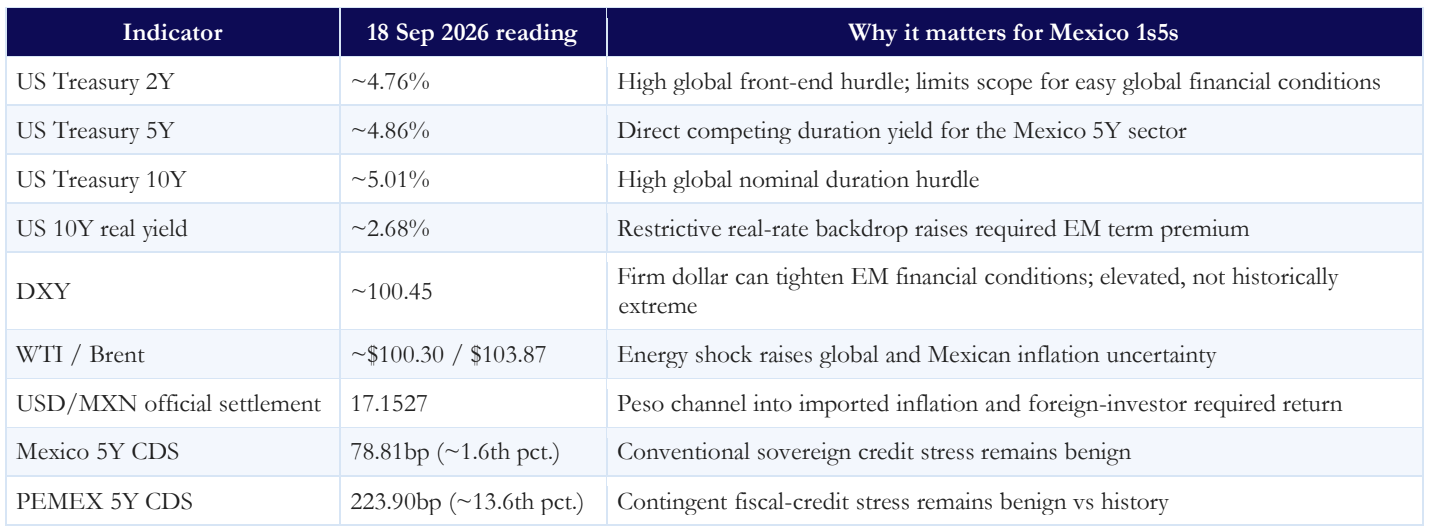
A global investor compares Mexican duration with the risk-free alternative available elsewhere. When US real yields rise, Treasuries offer more return without MXN currency or Mexican sovereign risk, so emerging-market bonds generally need to offer more compensation to remain attractive. A stronger dollar can tighten EM financial conditions further by increasing the potential FX loss on local-currency bonds and imported-inflation risk. Energy shocks can reinforce the same channel by keeping global inflation and developed-market yields higher.

That mechanism matters today. US nominal and real yields are high, the dollar is firm and oil has traded near $100/bbl, while Mexico-specific CDS remains benign. The current five-year premium can therefore be partly rational compensation for a difficult global duration environment rather than a Mexico-specific credit event. 

Hypothesis 4 – Foreign demand and positioning

A separate question is whether the marginal foreign buyer has withdrawn from Mexican duration. FX volatility alone provides little evidence: its contemporaneous relationship with 1s5s is weak. Direct holdings data are more informative. On 9 September, residents abroad held about MXN1.79tn of government securities, including roughly MXN1.51tn of fixed-rate Bonos. Foreign shares have edged down from end-2025, but the move does not resemble a disorderly liquidation large enough to explain a 99th-percentile curve on its own.

Offshore FX positioning provides a second, imperfect view of the marginal investor. CFTC data for 15 September show CME Mexican-peso non-commercial futures at 134,607 long versus 46,825 short contracts, a net long of about 87.8k contracts. In the Traders in Financial Futures classification, leveraged funds were net long roughly 90.0k contracts. Each contract references MXN500,000. This is evidence that speculative offshore FX positioning was still materially long MXN rather than positioned for an outright peso collapse; it is not a measure of local Bono duration positioning and should be treated only as a proxy. 

Hypothesis 5 – Cash-bond supply and liquidity

Cash-bond supply and liquidity remain plausible but incompletely identified. The 14 September official auction cleared the five-year Bono at 9.00%, while the 17 September vendor benchmark stood at 8.705%. The roughly 30bp difference is suggestive of a meaningful primary-versus-later-secondary gap, but it is not a clean auction-concession estimate because the observations are three days apart and we do not have the pre-auction when-issued/fitted yield for the exact security. A defensible concession study would compare the auction stop-out with a same-day pre-auction fitted or when-issued yield and then track post-auction performance. The evidence therefore supports ‘fresh primary-market cheapness exists’ more strongly than it supports a precise 30bp concession claim.

We therefore classify supply/liquidity as unresolved rather than force a regression from mismatched instruments. For trade monitoring, auction tails, bid-to-cover, dealer balance-sheet conditions, foreign holdings and any widening of Bono-versus-swap spreads should be treated as direct evidence that the premium is structural rather than a policy-expectations error.

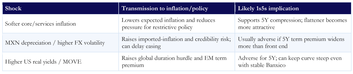
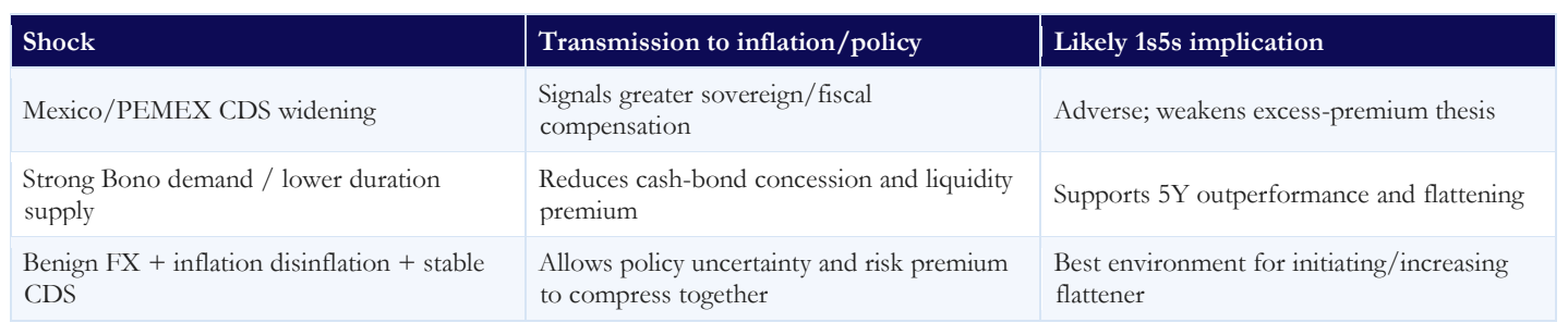
Synthesis: Cross-Asset and Macro Shock Map

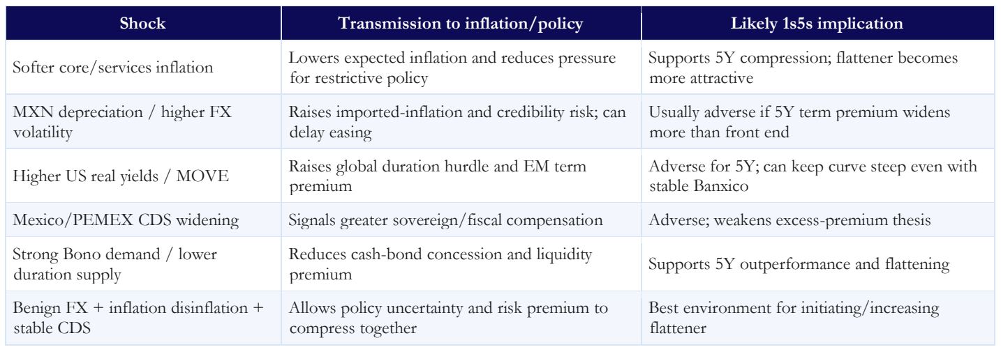
The relevant question for the flattener oncerns how shocks would move inflation expectations, Banxico and the five-year risk premium relative to the front end. Because the available aligned history is too short to identify a stable causal structural model, we do not estimate false-precision impulse responses. Instead we combine the observed survey distribution with the signs supported by monetary economics and the project’s empirical risk controls. This is a scenario-sensitivity model, not a claim of causal coefficients.

From Valuation to Trade: Constructing and Risking the 1s5s Flattener

The clean conceptual expression is receive/long the five-year Mexican rate and pay/short the one-year rate in matched-DV01 amounts. In cash, the long leg can be represented by a five-year Bono and the front leg by CETES or a short-duration hedge; in derivatives, the analogous expression is receiving fixed in the five-year MXN swap and paying fixed at the front end. 

Let D denote the matched DV01 on each leg. The first-order convergence P&L is shown below. With D = MXN10k per basis point, every 1bp flattening earns about MXN10k and every 1bp steepening loses about MXN10k before carry, roll and costs. From today’s 189.6bp spread, normalization to 150bp is a 39.6bp flattening and therefore about +MXN396k of curve P&L; 125bp implies about +MXN646k. Conversely, widening to 225bp costs about MXN354k and 250bp about MXN604k.

Using the 14 September auction yields as a transparent worked proxy, take the 363-day CETE at 7.24% as a one-year zero-coupon instrument. With MXN100 face value its approximate price is MXN93.25. Its Macaulay duration is one year, modified duration is about 0.9325 years, convexity about 1.74, and DV01 is about MXN86.95 per MXN1m of face value. For the five-year leg, because the exact reopened Bono coupon/cash-flow record is not in the supplied dataset, use a clearly labelled semiannual par-bond proxy with a 9.00% coupon and 9.00% yield. Its price is MXN100, Macaulay duration about 4.13 years, modified duration about 3.96 years, convexity about 19.45, and DV01 about MXN395.64 per MXN1m face value.

The hedge ratio is therefore about 395.64/86.95 = 4.55. A MXN10m face-value five-year position would be matched by roughly MXN45.5m face value of the one-year CETE proxy. If instead the risk budget is set directly at MXN10,000 DV01 per leg, the proxy notionals are about MXN25.28m face value in the five-year leg and MXN115.00m face value in the one-year leg. These large gross notionals are why DV01 should never be confused with capital committed or maximum loss.

Sensitivity is then easy to scale. At MXN10k matched DV01, a 10bp flattening is about +MXN100k, 25bp is +MXN250k, and 50bp is +MXN500k before carry, roll, convexity and costs. Halving the DV01 risk budget halves every one of those numbers; doubling it doubles them. This linear scaling is the simplest way to size the trade to a loss budget before considering second-order convexity effects.

A distribution, not a backtest

One historical episode gives intuition for what the distribution is summarizing. In May 2021 the monthly median 1s5s spread reached roughly 153bp, then narrowed by about 29bp over the following six months and about 50bp over twelve months. That episode is consistent with normalization after an extreme state, but it is not a template for today: the 2026 curve has reached materially wider levels and recent high-curve observations have been more persistent.

A mechanical backtest answers whether one fixed historical rule would have earned money. That is not the central question here. We instead estimate the empirical distribution of future changes in 1s5s and translate those changes into prospective P&L. The robust dataset uses monthly medians from September 2016 onward to reduce the impact of isolated bad daily prints. For each month we measure the subsequent 1M, 3M and 6M change in the spread. We report both the unconditional distribution and a high-curve distribution that only uses starting observations at or above the historical 80th percentile. The latter is closer to today’s valuation state without conditioning so aggressively that only a handful of episodes remain. A current-state conditional frequency is more relevant but uses fewer observations and is therefore less precise. We quantify that uncertainty with a 10,000-resample non-parametric bootstrap of the observed high-curve outcomes. We deliberately avoid imposing a Gaussian diffusion or presenting model-generated frequencies as certainties.

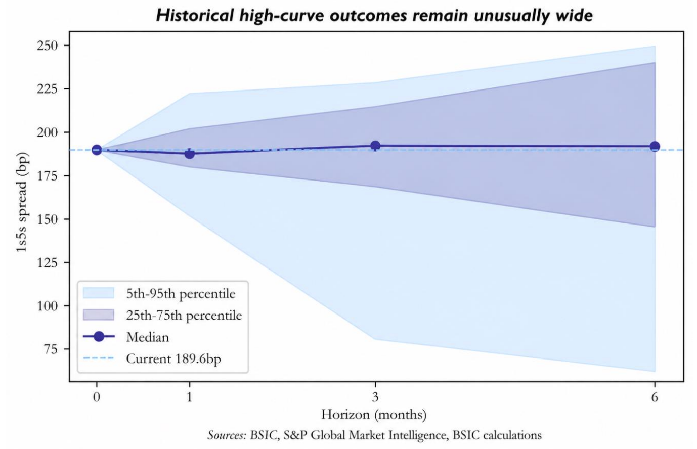
After high-curve starting states, the spread flattened in 62.5% of one-month observations, but only 45.5% over three months and 47.4% over six months. The 95% bootstrap intervals around those frequencies are wide – approximately 41.7-79.2%, 27.3-63.6% and 26.3-68.4%, respectively. At three months, only about 13.6% of high-curve observations would have taken today’s 189.6bp spread below 150bp, while about 9.1% would have ended above 225bp. At six months the distribution becomes much wider: about 26.3% reach below 150bp, but about 36.8% finish above 225bp. The historical evidence therefore indicates a large two sided distribution. The six-month asymmetry is the most important timing result in the paper: the historical high-curve sample was more likely to finish above 225bp (36.8%) than below 150bp (26.3%).

Conditioning additionally on benign sovereign CDS does not rescue the statistical case. The sample shrinks sharply, and the observed flattening frequencies are about 59% at one month, 40% at three months and 41% at six months. Because these are only 22, 20 and 17 observations, respectively, they should be treated as descriptive. 

Does the Result Depend on the Entry Threshold?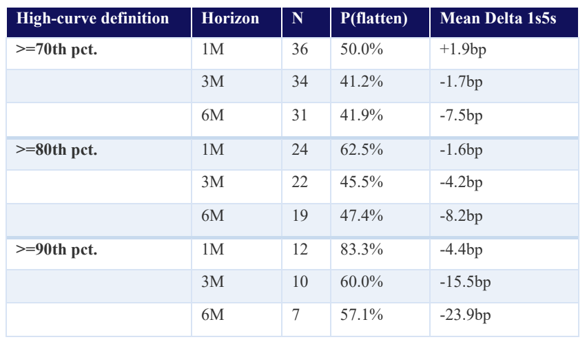

The results suggest that more extreme curve valuations contain some information about subsequent convergence, but not enough to define a reliable trading rule. At the 70th-percentile threshold, flattening is weak and inconsistent, while observations above the 90th percentile show larger average subsequent declines in 1s5s, reaching -23.9bp over six months. That said, this apparent improvement comes with a sharp reduction in sample size: the six-month 90th-percentile result is based on only seven observations. 

External-state conditioning and why we stop short of a precise probability

Ideally, the historical probability would condition simultaneously on today’s extreme 1s5s spread, elevated US real yields and energy prices, and benign Mexico CDS. The sample is too small to support that level of conditioning. The high-curve filter alone leaves only 24 one-month, 22 three-month and 19 six-month observations; adding further macro filters would reduce this to only a handful of cases. We therefore use the broader high-curve distributions as descriptive evidence rather than estimate a falsely precise probability for today’s exact macro state.

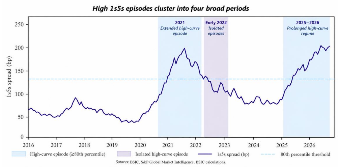
Even these observation counts overstate the independent information available. Months above the 80th-percentile threshold cluster into only four broad historical episodes, and the three- and six-month forward outcomes overlap within them. The 2025–26 regime is particularly important because, unlike several earlier high-curve episodes, it has not produced systematic subsequent flattening. Observation-level bootstrap intervals therefore do not fully account for dependence, while episode-level resampling becomes extremely imprecise with so few regimes.

Historically Calibrated Prospective P&L, Volatility and Tail Risk

Each realized spread outcome is mapped into P&L at a common MXN10k matched-DV01 risk budget using P&L approximately equal to minus DV01 times the change in 1s5s.. Longer-horizon observations overlap, so their effective information content is lower than the raw counts, and the 5% tail contains very few independent episodes. VaR and Expected Shortfall should therefore be read as transparent historical tail diagnostics for sizing today’s trade, not as regulatory capital estimates or forward guarantees.

Before quoting risk numbers, define the object being measured. Each historical or resampled future spread change is converted into a curve P&L using the chosen matched DV01. For MXN10k DV01, a +20bp steepening becomes approximately -MXN200k and a -20bp flattening becomes +MXN200k. The collection of these hypothetical P&Ls forms an empirical P&L distribution. Its standard deviation is the P&L volatility: a measure of how widely outcomes vary around their mean, not a worst-case loss.

Value at Risk asks for a percentile of that loss distribution. A 95% VaR is the loss threshold exceeded by only the worst 5% of observations. If 95% VaR is MXN386k, the historical conditional sample says that about 95% of outcomes lost less than MXN386k and about 5% lost more. It does not mean MXN386k is the maximum possible loss.

Expected Shortfall goes one step further. Instead of stopping at the 5th-percentile cutoff, it averages the losses in that worst 5% tail. Thus a 3M 95% Expected Shortfall of about MXN574k means that, among the most adverse 5% of historical conditional outcomes, the average loss was approximately MXN574k for a MXN10k-DV01 risk position. ES is therefore more informative about tail severity than VaR, but both remain sample-dependent historical statistics rather than guarantees.

For MXN10k of matched DV01 per leg, the empirical spread distribution maps one-for-one into curve P&L: a 25bp flattening is approximately +MXN250k and a 25bp steepening is approximately -MXN250k. Using the high-curve historical sample, expected curve-only P&L is approximately +MXN16k at one month, +MXN42k at three months and +MXN82k at six months. Those positive means are small relative to the dispersion: corresponding P&L volatilities are approximately MXN202k, MXN454k and MXN626k.

Tail risk is equally important. On the same curve-only basis, the empirical 95% VaR is approximately MXN322k at one month, MXN386k at three months and MXN589k at six months; 95% Expected Shortfall – the average loss among observations beyond the 5% VaR cutoff – is approximately MXN382k, MXN574k and MXN763k. These numbers are not capital-model VaR estimates: the sample is small, overlapping at longer horizons, and regime-dependent. They are transparent historical stress statistics that show the scale of adverse curve moves per MXN10k of DV01.

These tail statistics are historical diagnostics rather than stable population estimates. At six months only 19 qualifying observations remain before accounting for overlapping horizons and regime clustering, meaning that a 5% empirical tail is effectively determined by approximately one extreme raw observation. Six-month Expected Shortfall should therefore be interpreted as an illustrative stress measure rather than as a precisely estimated tail expectation.

Carry, roll and implementation matter

The distribution above intentionally isolates curve convergence. Carry and roll can materially change the economics, and the available benchmark-yield history is not sufficient to calculate exact security-level carry for a live Bono/CETES package. The cash implementation is especially important here because the one-year CETE is a discount instrument: it is purchased below par and mechanically accretes toward MXN100 at maturity. If the trade requires roughly 4.55 times as much front-end face value as five-year face value to match DV01, shorting that large amount of CETES means paying away their accretion. Thus, the simple cash proxy produced strongly negative carry in the earlier calculation. 

Execution costs should also be treated as first-order inputs. A 2022 IMF assessment described Bonos M as Mexico’s most liquid government-bond segment and reported an average bid-ask spread around 4bp, while a CFTC market-practice filing for MXN F-TIIE swaps describes a typical bid/offer around 3bp. These are historical/order-of-magnitude liquidity references, and are useful precisely because they show that a 10-20bp expected curve move cannot be evaluated without dealer-level execution, repo/funding and collateral economics.

The first alternative is a DV01-neutral MXN swap flattener. Instead of buying a five-year Bono and shorting a very large amount of one-year CETES, the investor uses interest-rate swaps: receive the fixed rate on the five-year leg and pay fixed on the one-year leg, sizing the two swaps so their DV01s match. If 5Y rates fall relative to 1Y rates, the value of receiving the now-above-market 5Y fixed rate rises more than the short-end payer leg loses, so the package profits from flattening. 

The second alternative is optionality. A 5Y receiver swaption gives the holder the right, but not the obligation, to enter a five-year receive-fixed swap at a pre-agreed strike on or before expiry. It therefore gains value if five-year swap rates fall sufficiently, while the maximum loss for the option itself is the premium paid. To target the curve rather than an outright 5Y rally, a desk can combine that receiver with front-end payer exposure or structure a conditional curve option so that payoff depends more directly on 5Y outperforming 1Y. This defined-loss structure is attractive when the empirical distribution has a wide adverse tail.

What would change this thesis?

The 24 September Banxico decision did not provide the simple confirmation a flattener thesis might have expected. Policy remained at 6.50%, yet the macro curve stayed steep while the local 5Y cheapness identified at research inception largely disappeared. This suggests that the 1s5s slope cannot be interpreted as a single temporarily cheap 5Y bond and instead contains a substantial front-end and broader term-premium component. 

Evidence for convergence would strengthen if inflation expectations, fiscal risk, MXN and global duration conditions improve while the curve remains extreme and the 5Y again becomes cheap relative to surrounding maturities. Conversely, persistent steepness after local 5Y residuals normalize would support a more persistent term-premium regime. 

Several limitations constrain these conclusions. Historical analysis uses S&P benchmark yields rather than security-level prices and cash flows, with robust monthly aggregation used to limit the effect of occasional bad daily prints. The effective sample is also smaller than the monthly count suggests because extreme states cluster into a few episodes and forward horizons overlap. Convergence appears stronger at more extreme thresholds but sample size falls rapidly, while stationarity is specification-sensitive for the regression residual and more robust for the leave-5Y-out Nelson–Siegel residual than for raw 1s5s. Finally, benchmark yields are not zero rates, Nelson–Siegel forwards are indicative rather than arbitrage-free, and the dataset lacks historical executable swap, repo and option economics. 

Conclusion

The evidence ultimately supports a narrower thesis than the original 1s5s valuation signal suggested. At research inception, the curve was close to the 99th percentile of its 2016–2026 history, but the roughly 190bp 1s5s slope was never equivalent to a 190bp five-year mispricing. The bond-specific models identified only 8-25bp of local 5Y cheapness, while raw 1s5s failed to establish robust stationarity. Structural-break tests reinforce that distinction: the macro slope can persist across changing regimes, whereas the leave-5Y-out Nelson–Siegel residual displays considerably stronger historical mean reversion. The conditional distributions tell the same story. More extreme starting states are associated with greater subsequent flattening, but observations are few, clustered across a small number of episodes and overlapping at longer horizons. Extremeness therefore contains some convergence information, but not a stable probability forecast.

The post-meeting evidence provides the clearest test of that distinction. The surrounding-curve regression and leave-5Y-out Nelson–Siegel diagnostics moved from approximately +24.5bp and +8.3bp of cheapness at research inception to roughly −14bp and −16bp, respectively, while the 3s5s10s fly compressed from about +69bp to +22bp. The persistence of macro steepness after local 5Y relative value normalized argues against interpreting the entire curve as one temporarily mispriced bond. Instead, a substantial part of the remaining premium appears associated with the front-end shape and broader macro term-premium regime.

The 3Y move is particularly instructive in retrospect. The latest cross-section places the 3Y around 8.09%, substantially above the 7.38% level in the research-inception, while the quoted 5Y remains near 8.71%. This change reveals what the original 1s5s framing obscured: much of the subsequent adjustment occurred inside the curve rather than through a 5Y rally. The 3s5s slope has compressed sharply and the current curve concentrates much of its steepness between 1Y and 2Y. In that sense, the analysis may have focused too heavily on the 5Y as the tradeable anomaly and insufficiently on the possibility that the more important relative move would come through repricing of the 2Y–3Y sector. 

Implementation makes the original flattener still less compelling. On the common MXN10k-DV01 scale, historical conditional mean convergence P&L is only approximately MXN16k, MXN42k and MXN82k at 1M, 3M and 6M, compared with illustrative cash-package carry of approximately −MXN0.40m, −MXN1.19m and −MXN2.39m. The cash implementation is therefore inefficient even if the directional view is correct. An MXN swap flattener could improve those economics, while receiver swaptions or receiver spreads can define downside, but neither can be judged attractive without live swap, funding and volatility pricing. 

The final result is therefore not that Mexican duration is demonstrably mispriced, nor that the current steepness must represent a permanent new regime. The evidence establishes something more precise: the macro curve is historically unusual; local five-year relative value is smaller, time-varying and model-dependent; and predictable convergence of the broader slope is not established. The first post-inception observation already demonstrates why those propositions must remain separate. A future position should therefore depend on renewed local relative value, supportive macro catalysts and executable carry rather than the 1s5s percentile alone. The broader lesson is that cheapness identifies where to investigate; it does not, by itself, identify the trade.

References

[1] Banco de Mexico, “Representative Interest Rates,” Sistema de Informacion Economica, accessed 18 September 2026.

[2] Instituto Nacional de Estadistica y Geografia (INEGI), “Indice Nacional de Precios al Consumidor y sus Componentes,” August 2026.

[3] Banco de Mexico, “Expectativas de Inflacion para los Proximos 12 Meses,” Encuesta sobre las Expectativas de los Especialistas en Economia del Sector Privado, August 2026.

[4] Banco de Mexico, “Quarterly Report April-June 2026,” published 26 August 2026.

[5] Banco de Mexico, “Mercado de Valores – Resultados de la Ultima Subasta de Valores Gubernamentales,” auction dated 14 September 2026, accessed 18 September 2026.

[6] Adrian, Tobias; Crump, Richard K.; and Moench, Emanuel, “Pricing the Term Structure with Linear Regressions,” Journal of Financial Economics 110(1), 2013, pp. 110-138; Federal Reserve Bank of New York Staff Report No. 340.

[7] S&P Global Market Intelligence, Mexico Rate Profile, Mexico Sovereign Credit Default Swaps Detail and Petroleos Mexicanos Credit Default Swaps Detail, proprietary data downloaded 18 September 2026.

[8] FactSet, Mexico economics and market-data snapshots supplied for this research, downloaded September 2026.

[9] Banco de Mexico, “Encuesta sobre las Expectativas de los Especialistas en Economia del Sector Privado: agosto 2026,” published 1 September 2026.

[10] Banco de Mexico, SIE CA227, “Expectativas de Inflacion Mensual,” August 2026 survey vintage.

[11] Banco de Mexico, SIE CA239/CR168, “Expectativas de la Tasa de Fondeo Interbancario,” August 2026 survey vintage.

[12] Banco de Mexico, SIE CR156, “Expectativas de Largo Plazo,” August 2026 survey vintage.

[13] U.S. Department of the Treasury, “Daily Treasury Par Yield Curve Rates” and “Daily Treasury Par Real Yield Curve Rates,” observations for 18 September 2026.

[14] Barron’s, “Dollar Rises to 7-Week High on U.S. Rate Hike Bets,” 18 September 2026.

[15] The Wall Street Journal, “Oil Futures End Week Little Changed,” 18 September 2026; WTI $100.30/bbl and Brent $103.87/bbl.

[16] Banco de Mexico, SIE CF102, “Daily Exchange Rates,” MXN per U.S. dollar, observations for 17-19 September 2026.

[17] Banco de Mexico, SIE CA175/CF457, “Tenencia de residentes en el extranjero / Tenencia de valores gubernamentales,” observations through 9 September 2026.

[18] S&P Global Ratings, “Mexico Outlook Revised To Negative On Weakening Fiscal Flexibility; BBB Foreign Currency Rating Affirmed,” 12 May 2026.

[19] Moody’s Ratings, Mexico sovereign rating action, Baa3 with stable outlook, May 2026.

[20] Fitch Ratings, Mexico sovereign rating affirmed at BBB- with stable outlook, April 2026.

[21] Banco de Mexico, “Calendario 2026 para los anuncios de las decisiones de politica monetaria,” next scheduled decision 24 September 2026.

[22] FactSet, “Yield Curve Analysis – Mexico,” benchmark yields as of 22 September 2026; Nelson-Siegel sensitivity and ridge robustness: BSIC calculations.

[23] U.S. Commodity Futures Trading Commission, Commitments of Traders and Traders in Financial Futures, Mexican Peso – Chicago Mercantile Exchange, positions as of 15 September 2026.

[24] International Monetary Fund, “Mexico: Financial Sector Assessment Program – Technical Note on Systemic Liquidity Management,” Country Report No. 22/338, 2022; reports average Bonos M bid-ask spread around 4bp in the cited sample.

[25] U.S. Commodity Futures Trading Commission filing, “F-TIIE Swaps,” market-practice summary; typical MXN F-TIIE swap bid/offer described as approximately 3bp.

[26] Nelson, Charles R.; and Siegel, Andrew F., “Parsimonious Modeling of Yield Curves,” Journal of Business 60(4), 1987, pp. 473-489.

[27] Bank for International Settlements, “Zero-coupon yield curves: technical documentation,” BIS Papers No. 25, October 2005.

[28] Cortes Espada, Josue Fernando; and Ramos Francia, Manuel, “An Affine Model of the Term Structure of Interest Rates in Mexico,” Banco de Mexico Working Paper 2008-09.

[29] Lelo-de-Larrea, Alejandra, “Forecast Comparison of the Term Structure of Interest Rates of Mexico for Different Specifications of the Affine Model,” Banco de Mexico Working Paper 2020-01.