Trading the Network II: What Should an Edge Mean?

Download PDF

Introduction

The first part of this study began from an intuitive proposition: financial markets are networks, and models capable of learning from those networks should therefore possess an informational advantage over models that treat securities independently. The empirical evidence was considerably less accommodating. A regularised linear model, Ridge regression, produced stronger out-of-sample forecasts than a conventional multilayer neural network, while both a Graph Convolutional Network and a Graph Attention Network deteriorated further. At the baseline specification, Ridge achieved a mean cross-sectional rank information coefficient of approximately 0.029, whereas the graph architectures produced values close to 0.01. Increasing the number of neighbours generally made the graph models worse rather than better.

The failure of a Graph Neural Network does not necessarily imply the absence of useful relationships between securities. A GNN is supplied with a particular graph constructed by the researcher. The economic meaning of an edge is therefore imposed before the neural network begins learning. If those edges represent the wrong relationship, additional computational sophistication cannot repair the underlying information problem.

Part I constructed edges from contemporaneous return correlation. If stocks i and j had moved together strongly during the preceding estimation window, they were connected. Mathematically, the relationship was based on

This definition captures similarity. It does not establish that movements in one security contain information about the subsequent return of another. Two companies can be highly correlated because both respond contemporaneously to the same market, sector, interest-rate or commodity shock. In such a case the statistical graph contains a strong edge even though no useful information flows from one company to the other.

Part II therefore asks a narrower question than Part I. Instead of asking whether a more complicated GNN can be made to outperform a simple model, it asks: what should an edge mean if the objective is prediction? The underlying equity universe, stock characteristics, forecasting target, walk-forward methodology, portfolio construction and transaction-cost assumptions are held constant. What changes is the definition and use of relational information.

Four graphs are considered: raw contemporaneous correlation, correlation after removing broad market and sector effects, directed lead-lag relationships, and directed lead-lag relationships estimated from residual rather than raw returns. In addition, a new model, Graph-Augmented Ridge, is introduced. Instead of asking a neural network to diffuse information across the graph, this model explicitly supplies a regularised linear regression with the stock’s own characteristics, information from its neighbours and the difference between the two.

Why Part 1’s Correlation Graph May Have Failed

The graph used in Part I was based on the Pearson correlation coefficient,

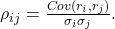
The problem is that a high value of ρ_(ij) has no intrinsic predictive direction. Suppose two stocks satisfy

where denotes the market return. Even if the idiosyncratic components and are completely unrelated, the two securities can exhibit substantial correlation because both load on the same market factor. The economic structure is therefore A←Market→B, rather than A→B. A correlation-based GNN nevertheless connects A and B and begins exchanging messages between them. The graph is statistically correct, but it may be predictively irrelevant.

Residualisation: Removing Common Information

Before abandoning correlation, we ask whether the problem arises because raw stock returns contain too much common market and sector information. Conceptually, each stock return is decomposed into

Here represents the broad market return, while represents the return of the sector to which stock i belongs. The coefficients and describe the security’s sensitivity to those common movements. The residual is what remains after the common components have been removed.

Instead of constructing an edge using , we can therefore use

This changes the interpretation of the graph. Two banks are no longer connected simply because the entire banking sector rallied. The residual graph asks whether the securities continue to move together after broad shared exposures have been stripped away. 

At the baseline k=3 specification, the residual-correlation Graph Ridge model produces a rank IC of approximately 0.02449 and an annualised return of about 11.21% with annualised volatility of approximately 18.70%. Its Sharpe ratio is approximately 0.661, modestly above ordinary Ridge’s 0.606, while its maximum drawdown is approximately -28.1% compared with Ridge’s -37.1%. This result is already revealing: a graph-derived representation can alter the risk structure of the trading strategy even when it does not improve average rank IC.

From Correlation to Lead-Lag

If the objective is forecasting, the natural relational question is not whether two securities move together at the same time. It is whether information in one security tends to precede movement in another. For a positive lag l, define

The arrow matters. The quantity asks whether returns in security j at time t are historically associated with returns in security i at a later time. An edge j→i therefore has a predictive interpretation: j is a candidate informational predecessor of i.

Part II evaluates several short lags,

and identifies the strongest historical predictive relationships within the available estimation window. This is conceptually different from contemporaneous correlation. measures similarity, whereas measures temporal ordering. Temporal ordering does not prove causation, because a third omitted variable could still generate both movements at different speeds. Nevertheless, a directed lead-lag edge is much closer to the economic mechanism required for a trading forecast.

Residual Lead-Lag: The Most Restrictive Graph

The strongest graph considered combines the previous two ideas. First, common market and sector effects are removed, so raw returns are transformed into residual returns. Directed relationships are then estimated using the residual components,

The resulting edge says approximately that, after removing broad market and sector co-movement, stock j’s idiosyncratic movement has historically preceded stock i’s idiosyncratic movement. The hypothesis is that, if relational alpha exists, it should be easier to detect when common information has been removed, and the graph is oriented according to predictive time.

The Key Innovation: Graph-Augmented Ridge

Part I left an identification problem unresolved. Suppose a GNN underperforms Ridge. There are at least two explanations: either the graph contains no useful information, or the graph contains information but the GNN processes it badly. Testing another GNN cannot cleanly distinguish these possibilities.

Part II therefore introduces Graph-Augmented Ridge. Let the stock’s own features be . For each stock, construct a weighted representation of its neighbours,

The weights are determined by the strength of the corresponding graph relationships. We then construct a third quantity,

This difference measures the stock’s network dislocation. The final feature vector becomes

Graph Ridge estimates

with the familiar Ridge objective

This architecture’s purpose is identification. If Graph Ridge beats Ridge, the graph contains incremental predictive information. If a GNN subsequently beats Graph Ridge, neural message passing adds value beyond simple graph-derived features. If Graph Ridge wins but GNN loses, relational information exists while conventional message passing is damaging it. The third possibility is precisely what the results suggest.

Why Network Dislocation May Matter More Than Network Average

The variable deserves particular attention. Suppose a stock has weak five-day momentum of 1%, while its strongest predictive predecessor has momentum of 5%. The relative signal is therefore

The economically interesting information may not be that the neighbour has risen by 5%, nor that the stock has risen by 1%, but that the stock has failed to participate in movement that historically tends to precede its own. This transforms graph information from an averaging mechanism into a relative-state variable. 

Graph Convolution Revisited

A Graph Convolutional Network updates node representations by mixing information across connected securities. A standard layer can be written as

The matrices à and D̃ respectively describe graph connectivity and normalisation by node degree. contains learned parameters, and σ is a nonlinear activation function. The crucial operation is multiplication by the normalised adjacency structure. Each node representation becomes partially composed of representations from neighbouring nodes.

This creates graph smoothing. If connected observations should resemble one another, smoothing can be extremely useful. However, cross-sectional trading rewards correct differentiation. The forecasting problem asks whether . Graph convolution can instead encourage when A and B are connected. This creates a potential mismatch between the inductive bias of the architecture and the economic objective.

Baseline Results at Three Neighbours

The primary Part II experiment initially uses three neighbours. Ordinary Ridge remains strong, with rank IC of 0.02893, Pearson IC of 0.02936, annualised return of approximately 11.66% and Sharpe ratio of 0.606. The ordinary MLP remains materially weaker, with rank IC of approximately 0.01789 and Sharpe of approximately 0.245.

Among graph-derived linear models, residual-correlation Graph Ridge performs particularly well economically. Its rank IC is approximately 0.02449, but its annualised return reaches about 11.21% with lower volatility of approximately 18.70%. Consequently, its Sharpe ratio is approximately 0.661, slightly exceeding ordinary Ridge. Its maximum drawdown is also considerably smaller, approximately -28.1% versus Ridge’s -37.1%.

The lead-lag Graph Ridge specifications do not beat ordinary Ridge at k=3. Raw lead-lag Graph Ridge achieves rank IC of approximately 0.02182, while residual lead-lag Graph Ridge reaches approximately 0.02510. At first glance, the lead-lag hypothesis therefore appears unsuccessful. The sparsity experiment changes that conclusion.

The Central Result: One Predictive Neighbour

When the residual lead-lag network is restricted to only the single strongest predecessor,

Graph Ridge produces the strongest predictive statistics in the experiment. Mean rank IC rises from ordinary Ridge’s 0.02893 to

This represents an improvement of approximately

Pearson IC similarly rises from 0.02936 to 0.03367, while the IC information ratio increases from 0.171 to 0.207. These three statistics point in the same direction. The improvement is therefore not merely a peculiarity of rank correlation: the model exhibits a stronger average association with subsequent returns and a better mean-to-variability ratio in its weekly IC series.

This result answers the first major question from Part I. Relational information can add predictive information. But it adds an important qualification: the useful relational information appears extremely sparse.

Why Residualisation Matters

At k=1, raw lead-lag Graph Ridge produces rank IC of approximately 0.02519. Residual lead-lag Graph Ridge produces 0.03284. Thus, removing common market and sector effects changes the lead-lag graph from one that underperforms ordinary Ridge into one that outperforms it on forecast quality.

Raw lead-lag relationships may partly identify delayed reactions to broad common shocks. The empirical improvement does not prove causal information transmission, but it strongly supports the narrower proposition that common-factor contamination matters when constructing predictive financial graphs.

Why Sparsity Matters

The strongest evidence in Part II is not merely that k=1 works. It is how rapidly the result deteriorates as neighbours are added. 

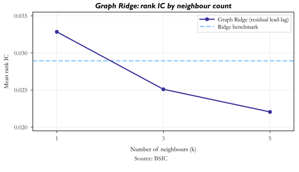
At one neighbour, Graph Ridge beats ordinary Ridge. At three neighbours, it no longer does. At five neighbours, performance deteriorates further. This is difficult to reconcile with the idea that financial relational information should simply be aggregated more broadly. Instead, the evidence supports an information-dilution interpretation.

The Decile Structure Confirms the Predictive Result

The k=1 residual lead-lag Graph Ridge predictions exhibit a clear cross-sectional relationship with realised returns. The lowest predicted decile subsequently earns approximately 0.183% over the five-day horizon, while the tenth decile earns approximately 0.645%. The upper half is particularly orderly: deciles six through ten earn approximately 0.296%, 0.351%, 0.408%, 0.504% and 0.645%, respectively.

The approximate top-minus-bottom spread is therefore

over five trading days before accounting for the precise long-short implementation and costs. The decile pattern is important because a positive mean IC could conceivably arise from a relatively small subset of observations. A reasonably ordered upper tail suggests that progressively stronger predictions correspond to progressively stronger subsequent returns.

The Crucial Negative Result: GNNs Still Lose

If the graph now contains useful information, a natural expectation is that a GNN should exploit it even better. The evidence rejects that expectation. At k=1, raw lead-lag GCN produces rank IC of approximately 0.01931. Residual lead-lag GCN produces 0.01625. Residual lead-lag GAT produces only 0.01151. By comparison, residual lead-lag Graph Ridge produces 0.03284.

The predictive hierarchy is therefore

Part I could not determine whether GNNs failed because graph information was useless. Part II shows that this explanation is insufficient. The graph can improve a simple model while still degrading a GNN. The problem therefore lies at least partly in how relational information is processed.

Why Attention Still Fails

One might argue that GAT should learn to preserve the useful neighbour and ignore irrelevant ones. At k=1, however, there is almost no neighbour-selection problem left. Each target has only one principal predecessor. Yet residual lead-lag GAT still produces rank IC of only 0.01151.

The failure cannot be attributed solely to attention being overwhelmed by dozens of bad neighbours. Instead, the nonlinear transformation and aggregation mechanism itself appears unnecessary or harmful. With one neighbour, the economically relevant structure may be sufficiently simple: own state, leader state and the difference between the two jointly predict the future rank. Ridge can estimate that relationship with relatively few effective parameters.

Random Graphs and Falsification

The random-graph experiments provide another important warning. At k=1, random residual lead-lag GAT achieves rank IC of approximately 0.01684, compared with 0.01151 for the genuine residual lead-lag GAT. Likewise, random lead-lag GAT produces approximately 0.01472, while real lead-lag GAT produces approximately 0.00957. These values should not be interpreted as evidence that random financial relationships possess economic information. Rather, they reinforce the conclusion that GAT performance cannot automatically be attributed to successful exploitation of the supplied graph

Prediction Improves, but the Portfolio Does Not

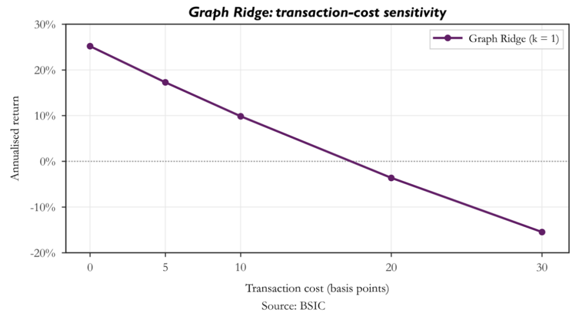
The strongest forecasting model does not produce the strongest net trading result. At k=1, residual lead-lag Graph Ridge achieves annualised return of approximately 9.86%, annualised volatility of 19.01% and Sharpe ratio of 0.590. Ordinary Ridge produces approximately 11.66% annualised return, 22.16% volatility and Sharpe of 0.606. Graph Ridge therefore improves predictive IC but slightly underperforms Ridge in net risk-adjusted portfolio performance.

The graph model has average turnover of approximately 2.519 per rebalance, compared with 2.145 for ordinary Ridge. Graph information changes rankings more aggressively. That can improve forecast discrimination while simultaneously causing more securities to enter and leave the long and short portfolios. The portfolio therefore pays more frequently to exploit the information.

Transaction Costs Explain the Forecast–Portfolio Gap

Before costs, the k=1 residual lead-lag Graph Ridge is substantially stronger. At zero basis points, annualised return is approximately 25.19% with Sharpe 1.278. At five basis points, return falls to 17.28% and Sharpe to 0.934. At ten basis points, annualised return is 9.86% and Sharpe 0.590. At twenty basis points, annualised return becomes negative at approximately -3.62%. At thirty basis points it falls to approximately -15.47%.

Performance Through Time

The sparse residual lead-lag strategy is also regime-dependent. Its net annual return is approximately -1.39% in 2018, 2.86% in 2019, 23.41% in 2020, -2.77% in 2021, 49.60% in 2022, 17.45% in 2023, 1.90% in 2024 and -2.62% in 2025. The strongest year is 2022, with a Sharpe ratio above 2.08. The strategy also performs strongly in 2020 and 2023, while it is approximately flat or negative in 2018, 2021 and 2025.

This pattern raises a further economic hypothesis. Lead-lag relationships may become more valuable when markets experience stronger cross-sectional propagation, dislocations or asynchronous repricing. In quieter environments, information may be incorporated too efficiently for delayed cross-stock relationships to remain economically meaningful. This regime interpretation should remain a hypothesis rather than a conclusion until explicitly tested.

What Has Actually Been Learned?

The combined Part I and Part II experiments allow several previously entangled hypotheses to be separated. The first hypothesis was that, because stocks are related, a GNN should outperform. Part I rejected this. Part II replaces it with the more precise proposition that some stock relationships contain predictive information. The k=1 residual lead-lag Graph Ridge result supports this proposition.

Part II suggests that financial graphs should not be thought of merely as maps of similarity. There are at least three different networks: a similarity network, an economic network and a predictive network. A similarity graph connects securities that behave alike. An economic graph connects securities through actual mechanisms such as supply chains, competition, ownership, financing or common inputs. A predictive graph connects securities where information in one historically helps forecast another.

These networks can overlap, but there is no reason they must be identical. For trading purposes, the third object is especially important. Our results suggest that a useful predictive graph may be extraordinarily sparse. For each security, perhaps only one relationship contains incremental information at a given moment. That interpretation is much closer to an information-transmission network than a broad similarity network.

Why More Connections Can Be Worse

Machine learning often encourages the intuition that more information should improve predictions. Statistically, this is false unless the incremental information possesses sufficient signal. Suppose

where S is the genuine predictive signal and ϵ is noise. Adding another variable Z helps only if its incremental relationship with S, conditional on the existing information, exceeds the estimation uncertainty it introduces.

Graph neighbourhoods face exactly this problem. The first edge is selected because it is strongest. The second is necessarily weaker. The third is weaker again. Thus increasing k mechanically lowers the average quality of the marginal edge. At some point,

Our empirical results suggest that this point may occur almost immediately. For residual lead-lag Graph Ridge, the optimal tested graph is not moderately sparse. It is the sparsest possible graph considered: k=1.

Statistical Significance and Caution

The improvement from an IC of 0.02893 to 0.03284 is economically interesting, but it should not be overstated. The absolute difference is only approximately 0.00391. Financial ICs are naturally small, but a modest improvement must still survive additional robustness tests before being interpreted as a durable anomaly.

Furthermore, k=1, k=3 and k=5 were all examined. Although these values were chosen for economically motivated reasons rather than through an unrestricted parameter search, model comparison itself creates some risk of selection bias. The correct interpretation is therefore that the evidence supports the hypothesis that sparse residual lead-lag information contains incremental forecasting value. It does not yet establish that a stable production trading anomaly has been discovered.

Conclusion

Part II began with a simple question: was the problem the graph, or the GNN? The answer is now considerably clearer. Part I’s contemporaneous correlation graph was not sufficient to establish that relational information improves forecasting. Once the network is redefined around directional lead-lag relationships and common market and sector movements are removed, a sparse graph does contain incremental predictive information.

At k=1, residual lead-lag Graph Ridge achieves rank IC of 0.03284 against ordinary Ridge’s 0.02893. Pearson IC and ICIR improve simultaneously. The graph therefore contributes information. But the GNN does not. GCN and GAT remain materially weaker than both Ridge specifications. The result suggests that conventional message passing imposes an inductive bias that is poorly aligned with a cross-sectional problem where relative dislocation may be more important than neighbourhood similarity.

The next experiment will preserve the winning k=1 residual lead-lag Graph Ridge model exactly as it is. Changing the forecasting model again would destroy the clean attribution achieved in Parts I and II. Instead, Part III will study turnover-aware portfolio construction. The central hypothesis is that the graph model contains superior information, but the strategy trades that information too aggressively. The research will then examine prediction persistence, rank buffers, entry and exit hysteresis, lower rebalance frequencies, confidence filtering and turnover penalties. 

References

[1] Kipf, Thomas N.; Welling, Max, “Semi-Supervised Classification with Graph Convolutional Networks,” International Conference on Learning Representations (ICLR), 2017.

[2] Velickovic, Petar; Cucurull, Guillem; Casanova, Arantxa; Romero, Adriana; Lio, Pietro; Bengio, Yoshua, “Graph Attention Networks,” International Conference on Learning Representations (ICLR), 2018.

[3] Feng, Fuli; He, Xiangnan; Wang, Xiang; Luo, Cheng; Liu, Yiqun; Chua, Tat-Seng, “Temporal Relational Ranking for Stock Prediction,” arXiv:1809.09441, 2018.

[4] Cheng, Rui; Li, Qing, “Modeling the Momentum Spillover Effect for Stock Prediction via Attribute-Driven Graph Attention Networks,” Proceedings of the AAAI Conference on Artificial Intelligence 35(1), 2021, pp. 55-62.

[5] Uddin, Ajim; Tao, Xinyuan; Yu, Dantong, “Attention Based Dynamic Graph Neural Network for Asset Pricing,” Global Finance Journal 58, 2023, Article 100900.

[6] Gupta, Gautam; Goel, Priyanshi; Verma, Divyanshi; Malhotra, Amarjit, “SGAT-SP: Sparse Graph Attention Networks for Stock Prediction,” Journal of Forecasting, 2026.

[7] Standard & Poor’s Dow Jones Indices, “S&P 500,” index methodology and constituent information; used here only as background for the large-cap US equity universe. Historical point-in-time membership is not reconstructed in Part I.

[8] BSIC calculations and backtest outputs for Trading the Network II. All reported IC, portfolio, turnover, cost-sensitivity and graph-density results are generated by the study described in this article.