Finding the Optimal Hedge for a Swap Maker’s Inventory

Download PDF

Motivation: Why go beyond dv01?

In the world of fixed income markets, hedging against interest rate exposure is one of the most essential aspects of risk management. This is especially true for market makers. Client trades leave the desk with exposure to rate risk across the tenors clients trade and due to adverse selection often also with risk which they don’t want to have on their book. If the desk has no particular view it wants to take, it will try to hedge their position and try to minimise the variance of the portfolio it’s holding on its book.

The simplest response could be to compress the whole book into a single number, its total DV01, and offset it with one liquid instrument, most naturally the 10Y gilt future in the case of Gilt and GBP rates desks. On days when the curve moves in parallel this works well as every tenor’s loss (gain) is offset by a gain (loss) on the futures position. However, it fails in two distinct ways. 

First, a single instrument at a single maturity hedges only the component of the portfolio’s P&L that co-moves with it. It cannot separately neutralise steepening, flattening, or curvature exposures: if the long end sells off while the 10Y point is unchanged, the portfolio takes the full loss with no offset. Second, a gilt future references the gilt curve, while a swap book’s risk lives on the SONIA curve, so the spread between the two markets passes directly into the hedged P&L. In practice, the future’s DV01 is not even a clean number, as it depends on which gilt is cheapest to deliver into the contract.

A better approach hedges with several instruments placed along the curve. This raises the question of which instruments to use, and the answer is dictated by liquidity as only a handful of benchmark maturities trade in real size. Hedging with every tenor would mean dealing in instruments with little depth, paying wide spreads for positions that are hard to adjust or exit. A small set of liquid benchmarks keeps the hedge executable and the estimates behind it stable. The task of this article is therefore to translate risk that lives between the benchmarks onto the instruments that trade at them.

Data and Portfolio Setup

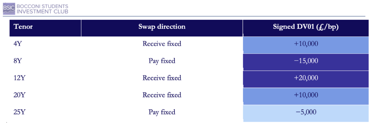
We construct a theoretical portfolio defined directly by its interest rate sensitivities: a received-fixed position with a DV01 of £10,000 per basis point at the 4Y, a pay-fixed position of −£15,000 at the 8Y, received-fixed positions of £20,000 at the 12Y and £10,000 at the 20Y, and a pay-fixed position of −£5,000 at the 25Y, for a net DV01 of £20,000 per basis point. Mixing paying and receiving positions mirrors a realistic dealer book, where client flow leaves exposures of both signs. The DV01 of a position is the amount, in pounds, by which its value changes when its yield moves by one basis point, and it is the natural unit for sizing hedges. The tenors are deliberately chosen away from the benchmark maturities, so no position can be hedged simply by taking the opposite side of a liquid instrument at the same tenor. The portfolio’s risk must instead be translated onto the benchmarks.

As hedging instruments, we consider the liquid points of the sterling market: benchmark SONIA swaps at the 2Y, 5Y, 10Y, and 30Y tenors, alongside the 10Y gilt future discussed above. Short-term SONIA futures offer an alternative, exchange-traded way to hedge the front end of the curve. For simplicity, we let the 2Y swap carry the front-end exposure in what follows.

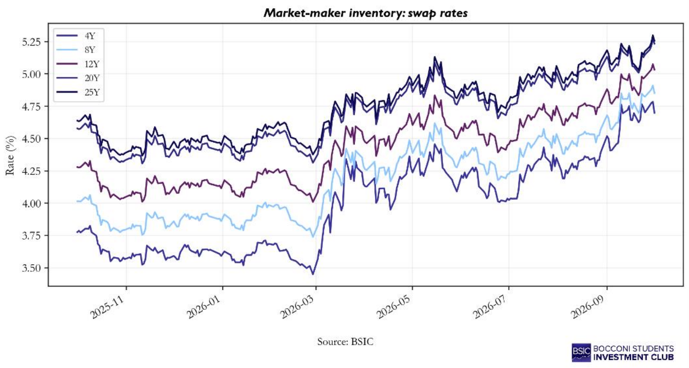
Our dataset consists of daily GBP SONIA swap rates across the curve, along with prices of the 10Y gilt future, from 1 October 2025 to 1 October 2026 (254 trading days). All analysis is carried out on daily changes in rates, measured in basis points, rather than on their levels. To measure the portfolio’s daily P&L, we rely directly on the DV01s: each position’s gain or loss is minus its DV01 multiplied by the daily change in its tenor’s yield, summed across the portfolio. Rising yields produce losses on received-fixed positions:

DV01s are signed, positive for received-fixed positions and negative for paid-fixed, so the same formula covers both sides of the book. This linear approximation captures most of the P&L for small daily moves, but ignores convexity, carry, and the gradual aging of the positions as their maturities shorten. Those effects would require a full repricing of each instrument, and they are one more reason the hedge must be rebalanced periodically, as discussed later in this article.

First Comparison: Hedging with the Ten-Year Gilt Alone

Aggregate DV01 matching

The simplest hedge compresses the book into its net +£20,000/bp sensitivity. A short gilt gains when its yield rises. Let be the gilt’s positive DV01 per £1m face at the previous close; the signed quantity held over interval t is: 

 

 

For example, £800/bp of sensitivity per £1m face requires a £25m short position. A common +1bp move approximately offsets the inventory’s £20,000 loss with the hedge’s £20,000 gain. This balances a specified parallel shock; individual tenor moves and changes in the swap–gilt relationship remain.

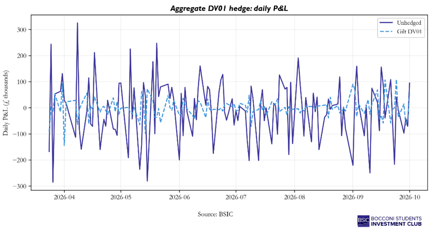
Figure 2. Daily inventory P&L before and after aggregate ten-year gilt DV01 matching. Source: BSIC calculations.

Rolling OLS with the same single instrument

Before broadening the hedge set, we ask whether statistical sizing improves the gilt hedge. Regress inventory P&L on the daily P&L G of one £1m long gilt unit over the previous 120 sessions. This estimates the historical co-movement of the whole inventory with the gilt, rather than imposing a one-for-one common rate shock. Using the same instrument separates sizing from instrument selection. One-predictor PCR retaining its only component would give the same fit as OLS.

Aggregate gilt DV01 reduces variance by 89.23%, compared with 90.69% for gilt-only OLS. Before applying more elaborate models, we next test DV01 hedges using swaps on the inventory’s own curve. This separates the change of hedge instrument from the subsequent choice of risk-mapping method.

Hedging with Liquid Swaps: DV01 Baselines

Aggregate DV01 in a ten-year benchmark swap

We can first neutralise the same net +£20,000/bp exposure using a liquid ten-year SONIA benchmark swap. A pay-fixed hedge with signed loss-DV01 of −£20,000/bp offsets the inventory’s net sensitivity to a common +1bp swap-rate move. Unlike the gilt hedge, this keeps the hedge on the inventory’s own rate curve:

 

 

This single-swap DV01 hedge reduces realised variance by 99.12% and leaves £10,778 of daily volatility on the same 133 dates. It avoids direct swap-gilt basis exposure but still compresses the entire book into one maturity and leaves non-parallel curve risk.

Allocating DV01 across all four benchmark swaps

A broader deterministic hedge maps each inventory tenor onto its two neighbouring benchmarks. If lies between and , allocate its signed DV01 in proportion to the distance from those maturities:

 

 

For example, the 4Y exposure is split one-third to 2Y and two-thirds to 5Y; the 8Y exposure is split 40% to 5Y and 60% to 10Y. Longer inventory maturities are allocated between 10Y and 30Y. Receiving and paying contributions net within each bucket before the opposite hedge is taken. The weights sum to one, preserving total signed DV01 by construction.

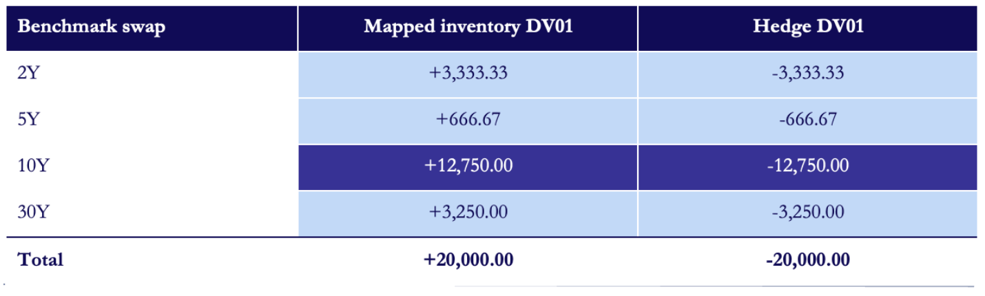
This is a maturity-based sensitivity allocation, not a full key-rate DV01 calculation obtained by bumping and repricing the curve. It exactly offsets common parallel shocks and shocks assumed linear in maturity, but actual curve movements need not satisfy either assumption. Its weights need no statistical estimation; they are fixed by the inventory and benchmark maturities. 

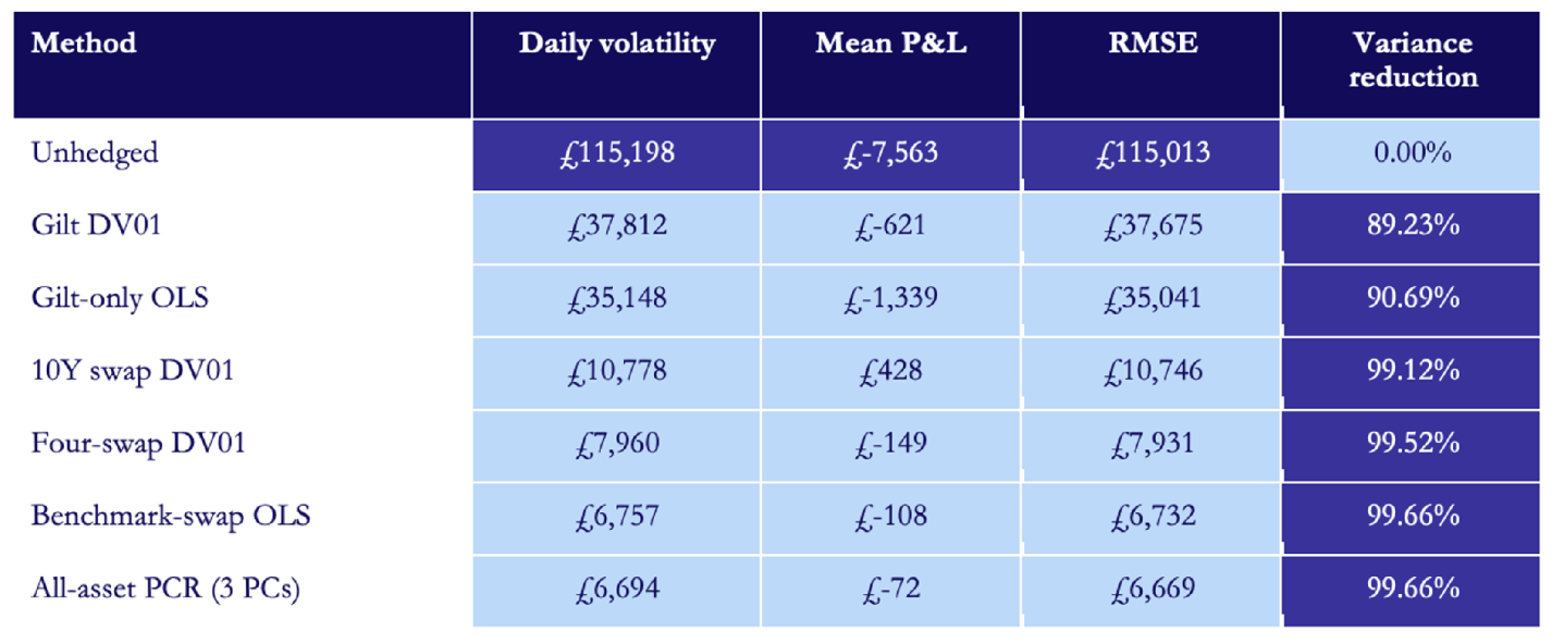
The four-swap DV01 hedge reduces variance by 99.52%, leaving £7,960 of daily volatility. OLS and PCR now have a directly comparable deterministic baseline within exactly the same four-swap universe: any further gain is a change in mapping, rather than the addition of new hedge instruments.  

Hedging with a Multiple OLS Regression

A better hedge begins with a better question. Before deciding how much to hedge, we need to know where the portfolio’s risk lives, expressed in the coordinates of the instruments available: an exposure at the 2Y, the 5Y, the 10Y and the 30Y, so that each piece can be offset with the corresponding liquid swap. These pieces are commonly called buckets. A deterministic alternative would split each position between its neighbouring benchmarks in proportion to maturity, the logic of key-rate DV01s. The regression approach generalises this: rather than imposing the split, it lets the observed co-movement of the curve decide it.

The tool is a multiple regression, applied tenor by tenor. For each off-benchmark tenor, we regress its daily rate changes jointly on the daily rate changes of the four benchmarks, over a rolling 120-day window:

Each beta measures how many basis points that tenor moves when a given benchmark moves by one basis point, with the other benchmarks held constant. It is essential that the four benchmarks enter one joint regression rather than four separate ones. Benchmark rates are highly correlated, and most days the whole curve moves together: a regression on any single benchmark would credit it with movements that in fact belong to the entire curve. In the joint regression, each beta captures only the contribution of its own benchmark after controlling for the others, and whatever the benchmark set cannot explain remains in the residual .

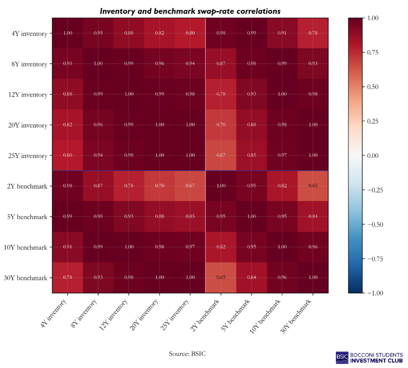
The heatmap below illustrates both the opportunity and the difficulty. Daily changes in swap rates are highly correlated across the curve, with each off-benchmark tenor moving closely with its neighbouring benchmarks, which is what makes hedging with a handful of liquid instruments possible at all; but the benchmarks are nearly as correlated with one another, and this multicollinearity is what makes the split of risk between them delicate.

The betas translate directly into risk. Each position’s DV01 is mapped onto the benchmarks through its loadings:

As an example, over the final window the 4Y rate loads 0.353 on the 2Y benchmark and 0.567 on the 5Y, so the 4Y position’s £10,000 of DV01 contributes roughly £3,530 to the 2Y bucket and £5,670 to the 5Y. Signs carry through: the pay-fixed 8Y position, loading 0.662 on the 10Y, contributes −£9,930 to the 10Y bucket, offsetting much of the +£14,860 contributed by the received-fixed 12Y. The book nets internally before anything is hedged. Repeating this for every position and summing produces the benchmark exposures in Table 1, and a useful check is that they sum to £20,286, almost exactly the portfolio’s net DV01 of £20,000: the regression redistributes the risk without inventing or losing any. The book’s first-order P&L now behaves approximately like these benchmark exposures, and each can be neutralised by paying fixed in the corresponding swap

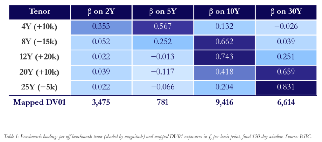
What the hedge cannot remove is the part of the original tenors’ movements that the benchmark regressions fail to explain. The residuals are exactly this: the curve bending between the benchmark points, the 8Y cheapening against both the 5Y and the 10Y with no benchmark combination responding. Even with all mapped buckets neutralised, the book retains this regression residual risk, and the hedge’s effectiveness depends on the estimated relationships remaining stable.

That stability is the method’s main caveat. Because the benchmarks are highly correlated, the split of a tenor’s risk between neighbouring benchmarks is delicate, and individual betas can shift as the window rolls even when the combined hedge performs well: over our sample, the risk mapped to the 10Y bucket roughly doubled, from about £4,500 to £9,000 per basis point, while the 5Y bucket shrank to near £1,000, with the portfolio itself unchanged, as the chart below shows. A short estimation window also risks fitting noise rather than relationships. The remedy is periodic re-estimation and rebalancing, which costs bid-offer on every adjustment: a trade-off between a tight, expensive hedge and a cheap one that drifts out of line.

Rolling betas and mapped exposures

The rolling 8Y betas below are directly interpretable in bp per bp and are the same coefficients used in the tenor mapping. Conditional betas may be negative or exceed one when predictors are correlated; they are not probabilities. An individual coefficient can change markedly while the combined fitted curve exposure changes much less.

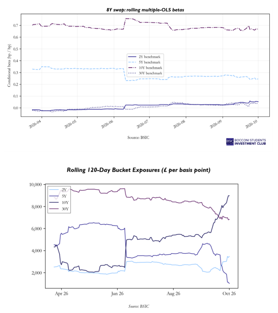
What the hedge cannot remove is the part of inventory-rate movements that the benchmark regressions fail to explain: for example, the 8Y point moving relative to the 5Y and 10Y benchmarks. Even after the mapped exposure is offset, regression residual risk remains. Re-estimation adapts the mapping, but changing coefficients generates rebalancing, whose bid-offer and other execution costs are excluded here.

Multiple OLS reduces realised variance by 99.66% and leaves £6,757 of daily volatility. This is performance after estimation, rather than a training-window goodness-of-fit statistic.

Understanding PCA: Common Movements and Factor Coverage

PCA replaces correlated observations with orthogonal combinations ranked by explained variance. On a yield curve, common-sign rate coefficients often describe level, short-versus-long signs slope, and the belly moving against the wings curvature. Those economic interpretations must follow the estimated shapes rather than the component number.

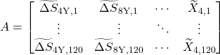
Our universe contains five inventory rate changes and four benchmark receiver-swap unit P&Ls. Let A be their centred observation matrix, with a tilde denoting subtraction of the corresponding column mean. The sample covariance matrix contains variances on its diagonal and pairwise covariances off the diagonal:

 

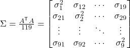
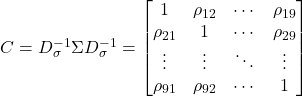
Let be the diagonal matrix of sample standard deviations. Standardising each column gives , whose covariance is the ordinary correlation matrix C. Every diagonal entry is one; each off-diagonal entry is covariance divided by the two standard deviations. Every series receives unit variance, without extra weighting between inventory and benchmark blocks.

 

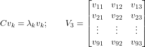
Order eigenvalues from largest to smallest and retain three unit-length eigenvectors. Multiplying the standardised observations by the eigenvector matrix produces three historical scores. Their sample covariance is diagonal:

 

 

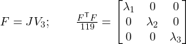
The first window’s three components explain 91.83%, 7.89% and 0.18% of joint standardised variance, or 99.89% together. The benchmark coordinates enter as receiver-swap P&Ls, so their signs are reversed relative to benchmark rate changes. The economic factor shapes must be interpreted with that sign convention. The correlation heatmap above displays rates on both blocks for easier comparison.

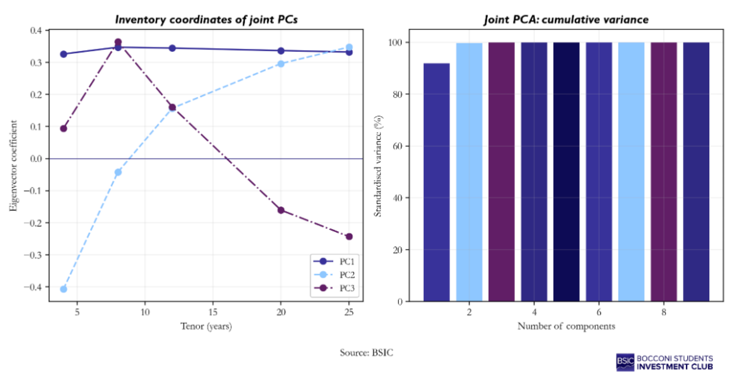
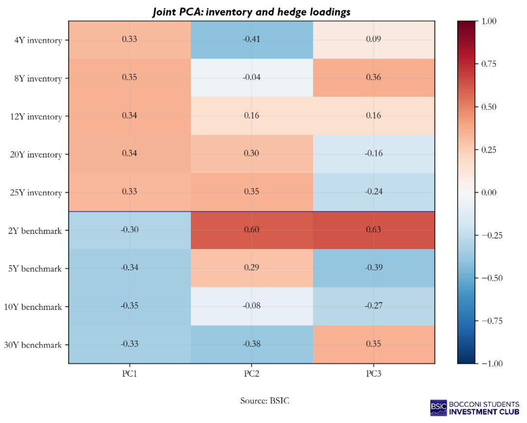
A high explained-variance share describes the joint observations; it does not equal the percentage of inventory P&L removed by an implementable hedge. A mixed-sign book may be sensitive to a low-variance curve direction, and benchmark instruments must still reproduce the retained factors.

Hedging with All-Asset Principal Component Regression

Ordinary benchmark-only PCR extracts factors from the hedge predictors and regresses inventory P&L on their scores. Retaining all independent predictor components recovers OLS; retaining fewer trades flexibility for dimension reduction. Our version instead extracts three components jointly from the inventory and benchmark observations, then implements them using only the four benchmark swaps.

The joint scores are statistical combinations, not instruments that can be traded. We fit centred inventory P&L on the three scores and regress those scores on standardised benchmark receiver-swap P&Ls . The resulting matrix M describes how the benchmark set replicates the factors:

 

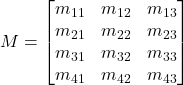
With the diagonal matrix of the four benchmark unit-P&L standard deviations, the combined regressions map factor exposure into signed benchmark hedge DV01:

Every mean, standard deviation, factor and regression coefficient is estimated from the previous 120 sessions.  Next-session hedge P&L comes from the fixed benchmark positions and actual subsequent benchmark rate changes. The five inventory tenors help estimate factors but never become additional hedge instruments.

Rolling factor participation of the eight-year swap

The 8Y swap’s first-window score correlations are 0.998, -0.036 and 0.046; its PC1 eigenvector coefficient is 0.347. For a standardised series, score correlation equals its loading multiplied by . Loadings describe participation in a factor, not hedge quantities.

Eigenvector signs are arbitrary. We align each vector with the preceding window by the inner product across all nine coordinates, reversing its sign and score when needed. Components remain variance-ranked. Sign alignment removes cosmetic reversals but cannot prevent rotations or crossings when eigenvalues are close.

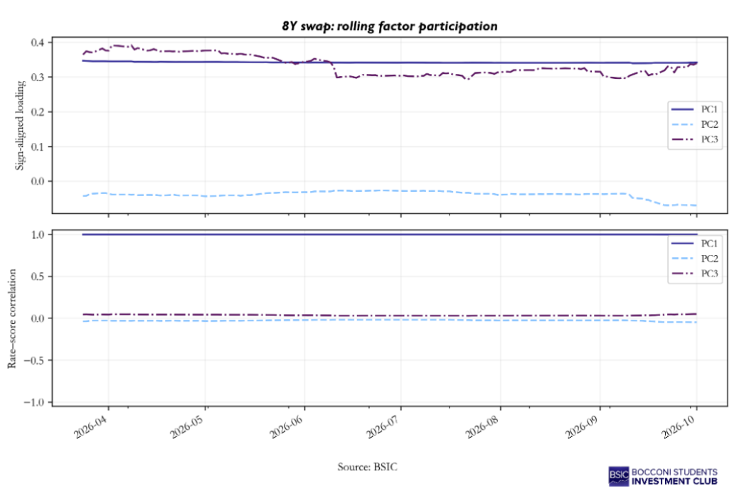
PCR reduces realised variance by 99.66% and leaves £6,694 of daily volatility. The final comparison assesses that compression against full multiple OLS.

Testing the Hedges: Variance Reduction

The practical aim is daily hedged P&L close to zero. We compare variance reduction and daily volatility on the same 133 dates, and report mean P&L and root-mean-square P&L (RMSE) to distinguish stability around a mean from closeness to zero. Variance measures dispersion around the sample mean; mean square equals variance calculated with denominator T plus the squared mean. No P&L series is demeaned or shifted in the displays.

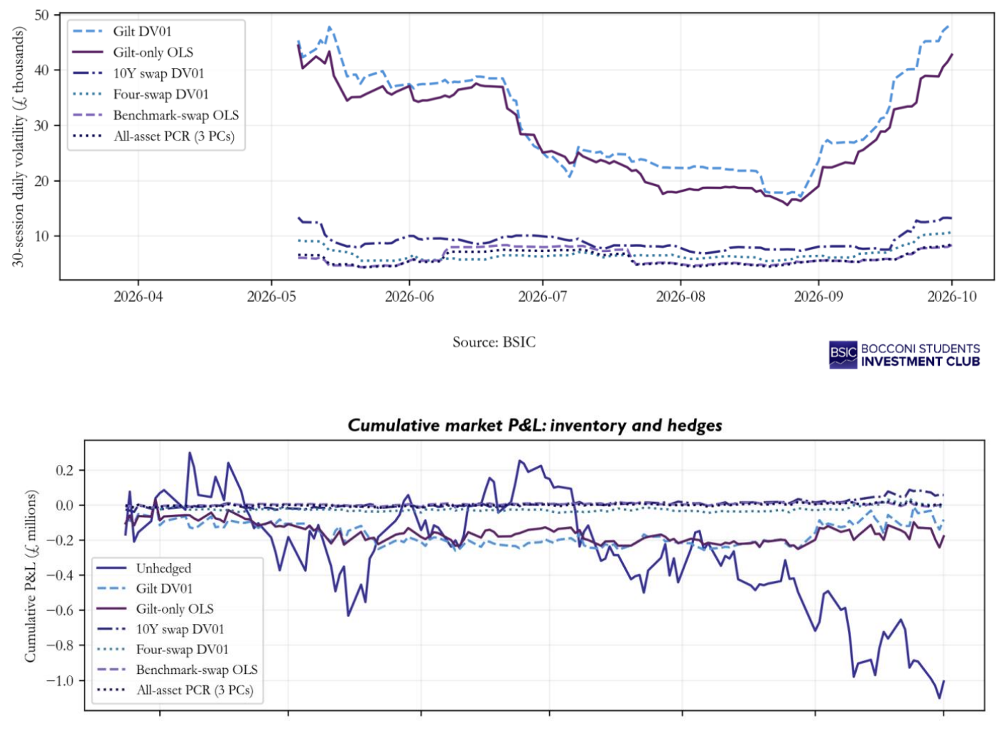
Concentration around zero indicates smaller daily gains and losses; the plotted P&Ls remain actual realised values.

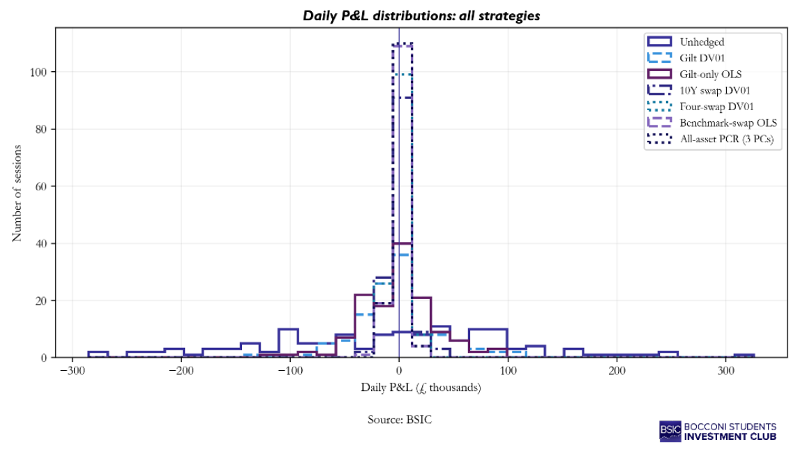
Figure 12. Cumulative market-driven inventory and hedge P&L. The lower panel expands all six hedged paths. Source: BSIC calculations.

Cumulative P&L shows how residual daily gains and losses accumulate. A positive terminal gain is not itself evidence of a better hedge. The comparison is based on dispersion and closeness of daily P&L to zero, rather than choosing the most profitable realised path.

What the model comparison tells us

The ten-year swap DV01 hedge removes 99.12% of variance, the deterministic four-swap allocation 99.52%, and OLS and all-asset PCR both 99.66% with a slight improvement on the latter. In volatility terms, the ladder is steep at the bottom and flat at the top: the gilt hedges leave roughly £35,000 of daily volatility, a single same-curve swap about £10,800, the four-swap allocation £7,960, and the statistical mappings £6,700–£6,800. Most of the improvement therefore comes from selecting instruments on the same curve as the underlying risk. Instrument selection determines which risks can be hedged; mapping only determines how well those instruments are allocated, and no statistical refinement can eliminate basis risk created by the choice of instruments.

PCA can represent slope and curvature through linear factors; non-linear modelling is not required simply because the yield curve bends. PCR may stabilise the hedge by discarding noisy directions but can also discard directions relevant to a mixed-sign inventory, while OLS retains all directions and remains sensitive to multicollinearity. Neither is guaranteed to perform better out of sample, and the three allocations tested, one fixed and two estimated, finish within 0.15 percentage points of one another. At this distance, the choice between them depends less on in-sample fit than on the stability of each method’s weights, the rebalancing they require, and their behaviour when the composition of the book changes.

Final hedge positions

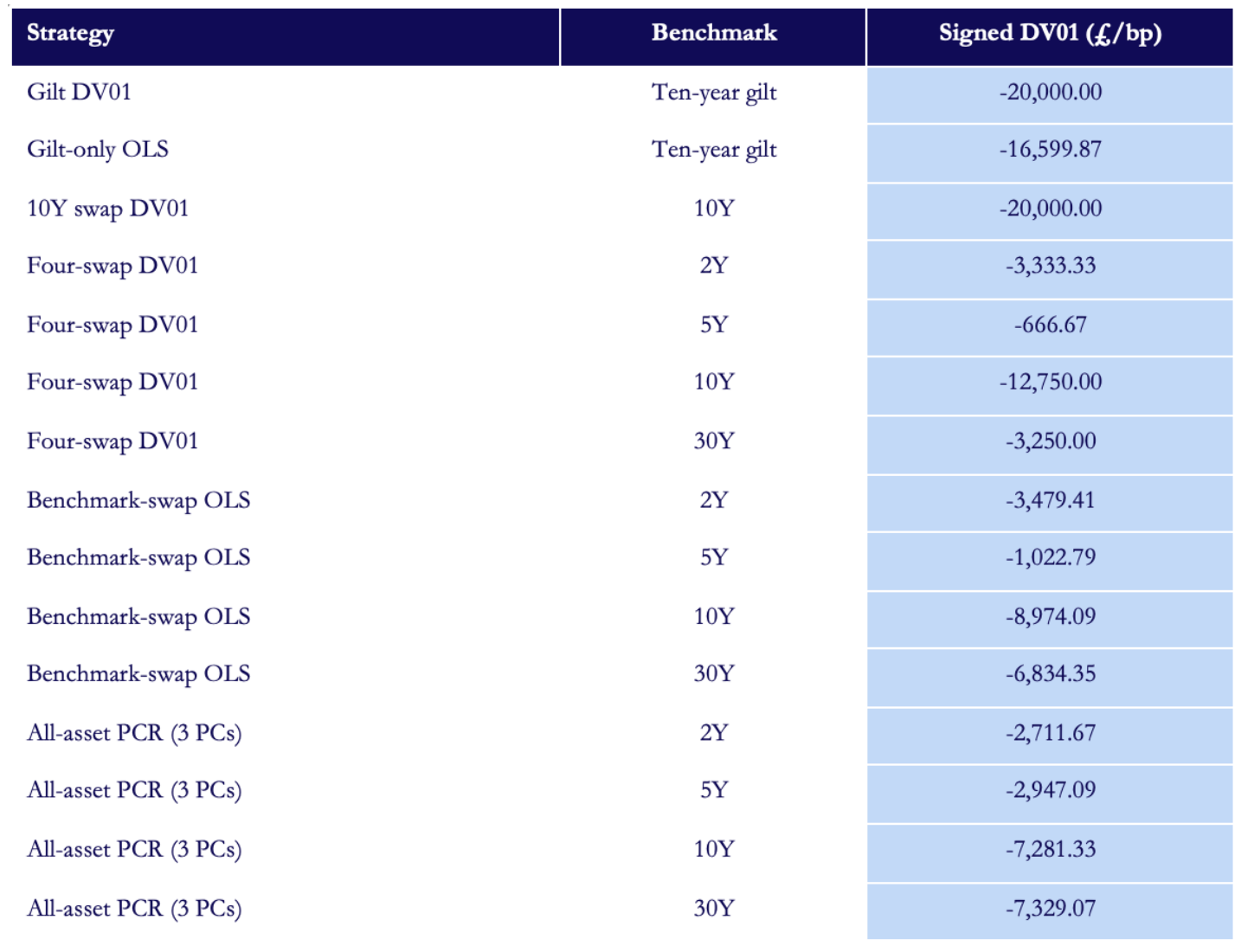
From a liquidity perspective, using standard 2Y, 5Y, 10Y and 30Y swap benchmarks is intended to concentrate hedging in commonly traded maturities with less capital required. A single ten-year hedge is simpler to execute, while four swap legs provide closer curve-risk matching but require more trades to establish and rebalance. Actual execution depends on bid–ask spreads, available market depth and trade size; the positions and hedge-variance results in this table do not measure liquidity or establish which strategy is cheapest to trade.

Conclusion and Implementation Limits

On this sample, the hierarchy of gains is unambiguous. Moving the hedge from the gilt future onto the inventory’s own curve removed most of the variance left by the cross-curve hedge. Spreading the hedge across four benchmarks removed close to half of the remaining variance. Choosing among deterministic, OLS and PCR mappings moved the result by little more than a tenth of a percentage point. Successive steps may, however, require more trades to execute or more estimates to maintain. 

The practical question is therefore not which method is most sophisticated, but where the marginal reduction in risk ceases to justify the associated implementation and rebalancing costs. For a desk, this means hedging on the right curve first, spreading the hedge across benchmarks second, and treating statistical mapping as a refinement to adopt only where its gains survive its costs.

The generic tenor-rate interpretation, fixed-DV01 approximation and modelled gilt delimit these results. A production test requires identified instruments, verified quote conventions and availability, executable notionals and trading costs. The benchmark choice expresses a liquidity rationale; liquidity itself is not measured here. 

Aggregate DV01 balances a specified common shock. Deterministic maturity allocation distributes sensitivity across benchmark swaps while conserving net DV01. OLS estimates that distribution from curve co-movement, and PCR compresses joint factors before mapping them into the same benchmarks. Their practical value depends on instrument coverage, relationship stability and the cost of maintaining the hedge.