From LIBOR to SOFR, the benchmark transition – Pt.4

Download as PDF

SOFR

On November 17, 2014, the Federal Reserve Bank established its own research group, the Alternative Reference Rates Committee, a commission composed by the major international banks, central counterparties and asset managers, with the support of the U.S. Department of Treasury,  the U.S. Commodity Futures Trading Commission (CFTC) and the Office of Financial Research (OFR). The group’s scopes were to identify a more resilient risk-free rate that would have substituted LIBOR in the US derivatives market, along with best practices for contractual resilience in the event of a cessation of its production. Also, the ARRC had to propose a transition plan with the guidelines for the adoption of this new benchmark. As a result of the consultation, they narrowed the set of potential alternatives to two kind of rates.

The first comprises overnight unsecured lending rates, namely the Effective Federal Fund Rate (EFFR) and the Overnight Bank Funding Rate (OBFR). The OBFR reflects overnight transactions in the Fed Funds market, as the EFFR, but also those in the Eurodollar one. Both are provided by the Federal Reserve, which collects data from over 150 banks for an average volume of around $70 billion per day in the Fed Funds market and $240 billion in the Eurodollar one. Nevertheless, the ARRC recognized flaws in both the alternatives: as the FSB already noticed, the Fed Funds market suffers from a scarcity of lending counterparties, and the EFFR is a policy target rate for the Federal Open Market Committee (FOMC). The OBFR would have been preferable for its broader underlying market. But transactions in this market are often arbitrage trades: some cash providers cannot earn the interest rate on excess reserves (IOER) deposited at the FED; thus they lend their money to institutions that can earn it, receiving back the OBFR or the EFFR, which are lower than the IOER. In this sense, the institution which earns the IOER and pays the OBFR/EFFR carry out an almost risk-free trade, namely an arbitrage trade.

The second possible solution was identified as the rate emerging from a set of repurchase agreements. Effectively, this is a market with high volumes and many transactions, and it had the possibility to provide a reliable risk-free rate. Repurchase agreements can differ for clearing procedures, collateral selection and other issues; thus, different segments of the market were considered. The first one is the tri-party repo market, in which there is a third-party agent who processes collateral selection, payment, settlement, custody and general management. Collateral is specified just at the end of the trading day: there is no requirement for specific securities (it is a cash-driven market).  For this reason, the collateral is usually of high credit quality: T-bills, notes and bonds, U.S. Treasury Inflation-Protected Securities, fixed and adjustable-rate mortgage-backed securities issued by Fannie Mae, Ginnie Mae and Freddie Mac, non-mortgage backed securities issued by government-sponsored enterprises and strips. Here money lenders are usually money market mutual funds and securities lenders. Borrowers are security dealers, who can use the money to fund their portfolios or settle other loans in the general collateral finance (GCF) repo market, which is a subset of the tri-party one. The difference between the two lies on the settlement procedures: usually, tri-party repos are not centrally cleared through a CCP, but the GCF ones are, with the benefits of higher liquidity and lower search costs. Another segment is the bilateral repo market, in which there is no third-party management, and the collateral is more precisely selected. Here, cash lenders are asset managers or security dealers and the borrowers are usually prime brokerage clients, such as pension funds, institutional investors and commercial banks. Even in this case, trades are generally not cleared through a CCP, except for a portion that is through the Fixed Income Clearing Corporation (FICC) Delivery-versus-Payment (DVP) service.

In the last years, repurchase agreements in these segments reached daily volumes around $800bn, making SOFR the money market rate with the highest number of underlying transactions. Since transactions underlying OBFR are just around $300bn in size, these measures supported the ARCC to create a rate based on the repo market. On June 22, 2017, the group announced the decision to produce and establish the Secured Overnight Financing Rate as a reliable alternative for the USD LIBOR. Since April 3, 2018, SOFR has been published by the Federal Reserve Bank of New York each business day around 8:00 am Eastern Time. SOFR is the average cost of financing Treasury securities overnight, and it arises from a volume-weighted averaged transaction-based calculation which considers transactions from:

• try-party general collateral repos secured by Treasury securities, which data are collected from BNYM, excluding trades made through the FICC GFC repo market and those in which the Federal Reserve is a counterparty;
• tri-party Treasury general collateral repo made through the FICC GFC market, for which the FICC acts as a central counterparty, collected from both BNYM and DTCC Solutions LLC;
• bilateral Treasury repos cleared through the FICC DVP service, collected from DTCC Solutions LLC.

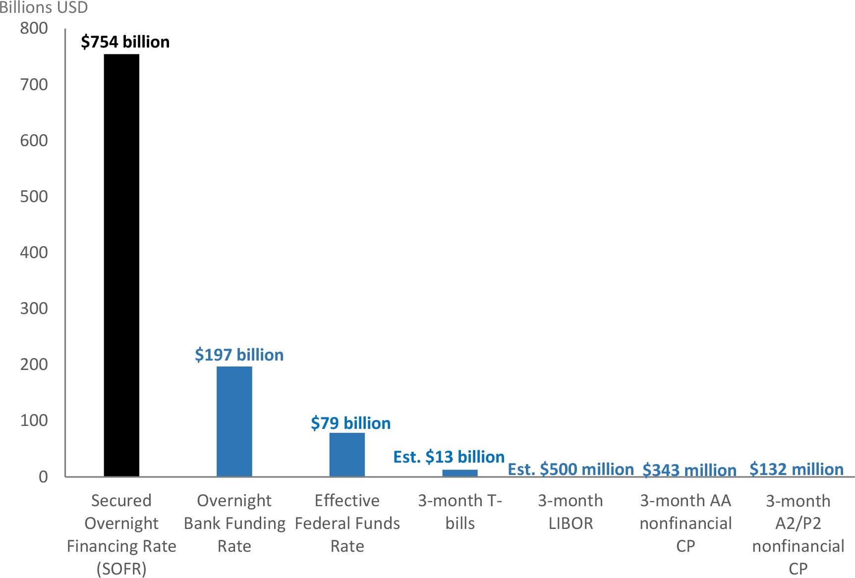
Daily transactions volumes in U.S. money markets. Source: The Alternative Reference Rate Committee

The calculation methodology consists in ranking the aggregate of repo trading volumes by their overnight transaction rates from the lowest to the highest and then calculate the transaction-weighted median repo rate, which becomes the day’s SOFR value, rounded to the nearest basis point. This means that half of the transactions is carried out at a rate above or equal to SOFR and half at a rate below or equal to it. Data are then filtered to be consistent with the IOSCO principles: for example, in the DVP repo market, the collateral is specifically selected before the trade. If an operator is looking for a particular security, he can accept a smaller return on the loan. As a counterbalance, DVP repo data with a rate below the 25th volume-weighted percentile rate are not considered in the calculation. As for ICE LIBOR, there is a precise procedure to follow if there are not enough transactions or if there is a mistake in the published value.

The graph below considers both overnight LIBOR and SOFR values between August 22, 2014, and August 17, 2018. During this period, LIBOR averaged 0.62%, and SOFR 0.67%: a mean difference of 5.01bps. SOFR seems less volatile than LIBOR (0.569 vs 0.576), but this is justified by the fact that LIBOR has periodically spiked following the variations in the EFFR. This has been, in turn, influenced by the changes in the FED’s policy rate that occurred on December 17, 2008, December 15, 2016, March 16, June 15, December 14, 2017, March 22 and June 14, 2018. To confirm this point, LIBOR volatility after the last FED change is equal to 5.67×10^(-5),  whereas SOFR one is 22.10. During these years, SOFR has been higher than LIBOR for 757 days out of 979, 77.32% of the time. The average positive difference is equal to 7.69 bps, whereas the average negative is -4.14 bps.

Overnight LIBOR vs SOFR. From August 22, 2014 to August 17, 2018. Source: Federal Reserve Bank of St.Louis; Federal Reserve Bank of New York

The Alternative Reference Rate Committee was also charged with the creation of a transition plan to migrate old and new contracts towards the new rate, to achieve an appropriate level of liquidity in the new derivatives market referencing SOFR, and to create a term structure for the reference rate. As a matter of fact, SOFR is an overnight rate. Thus, it can be easily integrated into interest rate swap and other derivatives: as the EFFR, it can be used in the calculation of the floating leg’s payoff of an IRS, possibly as a compounded average over a period of time. But credit products usually refer to a 1, 3, 6, 12-month rate or more, thus they need a forward-looking term rate, as it exists for LIBOR. For these reasons, the ARCC set up a Paced Transition Plan, with a specific timeline that should set the steps to entirely adopt the new rate. The plan, as reported in the Second Report (March 2018) required the participant banks to set up the proper infrastructure to begin trading futures and OIS in SOFR: trade data repositories, data providers and broader information systems needed to be adapted to the new rate; then, operators could begin trading uncleared products (by the end of 2018) and then the cleared ones (by the first quarter of 2019). Subsequently, SOFR should substitute the EFFR in two accounting practices: discounting and price alignment interest (PAI). The first consists in assessing the present value of the contract through a nearly risk-free curve. Instead, the price alignment interest is the overnight cost of funding collateral in a cleared interest rate swap trade. At the beginning of the swap life, each counterparty contract’s net present value (NPV) is 0, but with the subsequent variation of the floating rate, it changes. One of the two will have a negative NPV (out of the money), and the other a positive one (in the money). If party A has a negative NPV, it is obliged to pay this amount to the CCP, which will transfer it to party B. But the payment has to be funded, thus party A must also bear the cost of funding.  Party B, instead, will receive the NPV and, investing it, it will earn money. In order to rebalance the trade, the CCP obliges party B to pay a price alignment interest to the counterpart. This rate is chosen by the CCP, and until recent days it has coincided with the EFFR for USD derivatives.

The ARRC has proposed to gradually introduce the possibility to use SOFR in these two processes, as a stimulus to migrate to the usage of this rate. In essence, there was the necessity to have a SOFR term structure and thus an incentive for trading more and more contracts referencing it.

SOFR Futures

One of the steps toward the completion of this project was achieved the Chicago Mercantile Exchange, which on May 7, 2018, launched the first 1-Month (SR1) and 3-Month SOFR (SR3) futures, both as strips of respectively seven monthly contracts and twenty quarterly contracts. This means that there is always a 1-month future contract settling on one of each seven next months. Similarly, there are 3-months contracts for each of the next 20 quarters (settling on March, June, September and December), which allows for pricing the rate for the next five years. The SR1 settles each month for the next seven calendar month; its settlement price is equal to 100-R, where R is the arithmetic average of daily SOFR values during contract delivery month, rounded to the nearest 1/10th of a basis point. The contract unit is equal to $4,167 x contract-grade IMM Index, where the IMM index is 100-R, thus involving a value of $41.67 per basis point. The 3-Month futures, instead, settle each month on the morning of the 3rd Wednesday; the price-basis remains the same, 100-R, but the calculation methodology is different: here R is the business-day-compounded SOFR value during the contract reference quarter, calculated as:

Where:

• is the product of values indexed by the running variable, ;
• is the running variable indexing US government securities market business days during reference quarter;
• is the number of calendar days to which applies. SOFR is not calculated on Saturdays, Sundays and non-business days, therefore, in these cases, it is applied the last business day’s value in an accrued simple interest. For example, Friday’s SOFR value is extended to Saturday and Sunday, that means ;
•  is the SOFR value for i-th US government securities market business day;
• D is the number of calendar days in the reference quarter.

The formula is built following this logic:  is the rate multiplied by 100, thus it is converted in the right form (dividing by 100). Then it is divided by 360 and multiplied for the number of days to which it applies (). The result is a gross return. The final settlement rate is the result of the compounding of all the gross returns (that is multiplying them), multiplied by (360/D) and expressed as a percentage. The contract size is equal to , thus involving a value of $25 per basis point. For both SR1 and SR3, R is a measure of market expectations. In the first case, it is the expected value of the average daily SOFR during a precise month. In contrast, in the second case, it is the expected compounded rate during the reference quarter expressed on a 12-month basis. Of course, as the contract enters in its reference period and R starts to reference the published value, the uncertainty about the final settlement price decreases. Overall, market response to the introduction of these futures has been positive. During the first week (from May 7 to May 11), 7,263 contracts were traded with an open interest of 3,595 contracts. During the first ten days of trading, these numbers outpaced those of the Eurodollar and Fed Funds futures on their respective first teen days after launch. As of July, 30, open interest reached 23,383 contracts, while on August, 8, contracts traded since the first day amounted to 152,000. Along with futures, CME introduced new inter-commodity spreads (ICS). These products allow operators to bet on the difference between two similar assets. In this case, between 1/3-month SOFR and 30-day Federal funds or 3-month Eurodollar. Also, CME Group started clearing two kinds of OTC SOFR Swap: OIS swap that pays a fixed rate versus the compound SOFR, and four basis swaps that pay either 1-month, 3-month or 6-month LIBOR versus SOFR or the EFFR vs SOFR. Both these instruments are set to increase liquidity and facilitate price discovery.

The Last Developments

SOFR has already been adopted in cash products. On July 25, 2018, Fannie Mae, with the intermediation of Barclays Capital, Nomura Securities International and TD Securities, issued for the first time a $6 billion floating-rate note priced at SOFR. On August 14, 2018, the World Bank launched the first SOFR bond, raising $1 billion at 2-year maturity, with a quarterly coupon of SOFR + 22 bps. Then, on August 20, 2018, Credit Suisse issued a $100m certificate of deposit priced at 35 bps above SOFR, with a maturity of 6 months and, on August 30, the U.S. private insurer MetLife issued two-year floating-rate notes for $1 billion with a coupon of SOFR plus 57 bps.

The warm reception of the new benchmark should not make us forget what is still necessary to implement for the complete adoption of the rate. As we have already noticed, forward rates are still missing, but cash products usually reference them. Yet, there is the possibility for these to integrate the new rate as a backward-looking average. Still, the contract’s payoff would be determined at maturity, not at the beginning, as for LIBOR. Indeed, when the CME will introduce SOFR OIS, operators will manage to build a LIBOR-like payment structure: instead of paying a compound average of SOFR at the end of the period (for example 1 year), an investor could enter into an OIS, in which he periodically receives the compounded average of SOFR (for example quarterly) and pays back the 3-month LIBOR/EFFR. This methodology allows us to know the exact contract’s payoff at the beginning of the arrangement, but it is subjective about the existence of LIBOR. Besides, paying LIBOR over SOFR would probably be an inefficient idea, since SOFR, lacking the credit premium, trades lower than LIBOR.

Nevertheless, as the ARCC confirmed, there will be the possibility to build a forward term structure once the market in SOFR futures and OIS will be robust enough.

The proposed ways to recreate it would arise from trading in these contracts: a term rate could be constructed by bootstrapping between the prices of nearby SOFR futures contracts, or through a curve fit across all OIS transactions at a range of money-market maturities. There would be also the possibility to use actionable market quotes, that is a calculation through order books over a period of time, a method used for ICE Swap Rate.

Even once the term structure will be implemented, contracts referencing USD LIBOR cannot be simply migrated to the new risk-free rate (RFR). Such a procedure would be an economic imbalance, because moving a credit product benchmark from LIBOR to SOFR would merely mean reducing the amount of payments: the unsecured nature of the former requires a premium, that is absent in the latter. Nor it would be acceptable from a legal point of view, since contractual agreements may not allow for such variation.

In light of this, the announcement made by Andrew Bailey, FCA chief executive, stating panel banks will not be required to submit LIBOR after 2021, effectively compels to find out a path for a smooth transition. Even if the ARRC (as the other groups) has managed to find a new robust rate and create new contracts referencing them, it has not the power to impose a conversion method to all the agreements. Luckily, this work has been undergone by other institutions. As far as derivatives are concerned, the leading role is played by the International Swaps and Derivatives  Association (ISDA), which sets the contractual standards for transactions in these instruments. A part of its standardized agreements regards the fallback that will be applied in case of benchmark discontinuation.

In the past, these agreements were activated in case of electronic system errors, computer glitches or temporary market stress. Instead, now they must address a non-reversible situation. Thus, ISDA is revising them for solving the problem of a permanent benchmark cessation. Once the fallback triggered, following the publication of a public statement announcing it, the new rate will be required to adapt to the term structure of IBORs and to compensate for the difference between them and the RFR. The first adjustment is needed because of the overnight nature of the RFRs and of the current lack of a forward-rate curve. Even if ISDA considered the possibility to keep the overnight rate of the day proceeding the announcement, potentially in the convexity-adjusted form, it also proposed two other solutions:

1. A compounded setting in arrears rate, resulting from the compounding of the overnight RFR over the IBOR tenor, known only at the end of the period.
2. A compounded setting in advance rate, calculated as the former, but over the period immediately preceding the start of the IBOR tenor. Thus, it would be a backward-looking rate known in advance.

The subsequent modification wants to calibrate the economics of the rates, accounting for the credit-risk premium incorporated in the IBORs. Its equivalent should be added to the RFR, through one of these approaches:

1. The forward approach, which adds the forward difference between the specified term IBOR rate and one of the compounded RFR. The resulting value will be known in advance only if the adjusted RFR will have been set in advance.
2. The historical mean/median approach, in which the compensation is:
   1. the spot IBOR-adjusted RFR spread at the time of discontinuation,
   2. the mean or the median of the same spread, calculated over a significant past period of time (at least 5 years), after a year.

The linear interpolation of the two points would provide the compensation values for the transitional year.

3. The spot-spread approach. The added value would be simply the spot-spread between the rates one day before the triggering.

Regardless of the selected methodology, the replacement would (and probably will) recur only once. After that, there should be no derivatives referencing the old IBORs, whereas the new ones should have already started referencing the new RFRs. That said, the migration to the new benchmark, even if well prepared, will not exclude value transfers across counterparties. Also, it will be executable only if they both adhere to ISDA protocols. Non-adherent operators will need to amend on a counterparty-by-counterparty basis, making the entire transition more difficult, if not impossible. Unfortunately, this last issue is even more widespread in the credit market: being often individual arrangements, these products require more complex coordination for the migration, even because they frequently lack fallback provisions. The Loan Syndication and Trading Association (LSTA) is a member of the ARCC, and it is supervising and looking for possible solutions. Even if the methods proposed by ISDA for adding the credit spread to the RFR could even work for credit products, there is still no public recognition of this possibility. Different contracts are characterized by different fallback provisions and amendment practices. Syndicated business loan agreements can be usually changed with the consent of the majority of lenders, but floating rate notes’ terms can be adjusted only with the approval of all the note-holders, who sometimes are even difficult to locate. Agency securities and mortgages usually allow their issuer to select a successor rate in case of the benchmark cessation. But those securities which are not “agency” often require an unanimous consent.  The entire matter is compounded by the fact that firms may not want to face legal challenges arising from investors’ discontent with provisions’ changes. In this case, floating-rate instruments could become either fixed, referencing the last available LIBOR value, or pegged to the fallback determined by the old arrangements.

This question, along with those about building the proper infrastructure, reaching a higher level of liquidity, migrating discounting and PAI and calculating a term structure, are just a part of the adjustments to be undertaken. Market participants must actively take part in the transition process. They should measure both their exposure to the IBORs and the roll-off structure of their portfolio. Then, they should understand the possible impact of a rate cessation to their activity, keeping in mind that not only LIBOR but also the other interbank rates are going to be substituted. There is no guarantee that this process will follow a unique timeline. Thus, it is necessary to account for currency mismatches in the introduction of the new rates. Operators should also take into account possible mismatches in their balance sheets if assets and liabilities do not readily adopt the RFR at the same time and with the same tenor.

Both these last two situations give birth to basis risk: in this case, market participants should start asking and trading the new required hedging products. Besides, if assets reference the new rate before liabilities (or vice versa), there may be a reduction of the collateralization ratio, thus requiring more collateral to be posted. A revision of the accounting practices will be required too, as well as an understanding of the effects on taxation. Once the strategy has been established, market participants should communicate it clearly, defining a precise transition plan.

Conclusions

Financial market’s structural conditions require benchmarks to be revisited and innovated. The decline in unsecured interbank lending, the manipulation scandal and the massive discrepancy between the reference and underlying markets demand for a revision of LIBOR and the other IBORs. Under an administrative point of view, regulators have enhanced LIBOR’s submission, calculation and publication methodologies and their supervision. Nowadays, ICE Benchmark Administrator is responsible for all these processes. It has also created the new Waterfall Methodology, which wants the rate to rely more on transactions rather than judgments. Nevertheless, an enhanced LIBOR will not address the structural problems of its underlying market, nor it will be immune to the effects we have illustrated in the section. In addition, it is almost certain that the rate will disappear.  Therefore, the financial industry must take into account the likely future cessation of the benchmark. Effectively, new rates have been created. They are precisely calculated from deeper underlying markets, and they should be more resilient to market stress. But, as it has been widely noticed, the overnight and sometimes secured nature of these rates requires a precise adoption methodology. Practical guidelines must be provided to smooth the transition of old contracts to the new benchmarks. In this case, an efficient plan will reduce all the risks involved by such a change (litigation, contractual frustration, basis risk, balance sheet mismatches, etc.). New resilient rates have been developed, and SOFR has been warmly accepted in new products, but their different natures still require an enormous effort to become effective benchmarks. Global coordination between market operators, institutions and regulators is necessary to address the problem, bearing the minimum possible risk.