Poker as an imperfect-information game
In chess, both players see every piece and its position. Poker is different: although the community cards are public, each player’s hole cards are private. The opponent cannot directly observe our hand during betting. They see our actions and use them to draw conclusions about what we might hold. This makes poker a game of imperfect information, and it changes what a good strategy looks like.
Consider a bot that follows a simple, sensible-looking rule: bet with strong hands, check with weak ones. Against an opponent who does not adjust, this might perform well. But an attentive opponent soon learns that a bet always signals strength. They can fold more often against the bot’s bets and attack its checks. That reduces the money its strong hands earn and puts pressure on its weak ones. The rule has made the bot’s hand strength predictable. Bluffing too often creates the opposite problem: the opponent can profit by calling more often.
Rock-paper-scissors provides a simple illustration. Always playing rock loses to an opponent who notices and switches to paper. Randomising independently between rock, paper and scissors, with equal probability, removes that opportunity. The frequencies matter: a player who chooses rock most of the time is still exploitable, even though their choices are random.
Poker requires similar logic, although its probabilities depend on the hand and the betting situation. A strategy specifies how often to take each available action, given our private cards and the public betting history. Some hands may always bet, others may always check, and some may mix: for example, betting 70% of the time and checking 30%. The aim is not to stop the opponent learning anything from our actions. A bet will still make strong hands more likely in their eyes. The aim is to balance the hands behind each action so that the opponent cannot profit from a predictable imbalance.
Our previous article examined bet sizing and capital at risk through the Kelly Criterion, using estimates of equity and of the opponent’s responses. Here we ask how to build the playing strategy itself when the opponent can adjust to it. Which combination of value bets, bluffs and calls leaves the opponent no profitable adjustment? Answering that requires a precise concept of mutually optimal strategies: a Nash equilibrium.
Nash equilibrium and exploitability: what “GTO” means
A Nash equilibrium is a combination of strategies in which no player can improve their expected payoff by changing their own strategy while the other players’ strategies remain fixed (Nash, 1950). Each player’s strategy is a best response to the others’: given how they play, no alternative does better.
Consider heads-up poker without rake: there are two players, and one player’s gain is the other’s loss. Von Neumann’s minimax theorem (1928) gives such games an especially useful property. They have a value, and an equilibrium strategy guarantees at least that value in expectation against any opponent, not just one who also plays an equilibrium strategy. In this two-player, zero-sum setting, that guarantee is the protection offered by “game theory optimal”, or GTO, play.
Two clarifications prevent common misunderstandings. First, the guarantee concerns expected results, not any hand or session: a GTO strategy still loses many individual pots. Second, it guarantees the game’s value, not necessarily a profit. Some positions have negative value. In Kuhn poker, for example, the first player to act expects to lose 1/18 of a chip per hand when both players play perfectly. When the game is played from both positions equally often, these positional advantages cancel out.
In small games exact equilibria can be computed, but in large poker games the strategies we compute are approximations, so we need a measure of how vulnerable they are. Exploitability is the additional expected payoff that a best-response opponent could earn against a strategy, beyond that opponent’s equilibrium value. The opponent is assumed to know our strategy, including all its action probabilities, but not to see our private cards. An equilibrium strategy has zero exploitability; a larger number means a best response could extract more, although a real opponent may fail to spot or use the weakness. When we evaluate a complete strategy profile, our implementation averages this vulnerability across the two players and reports it in chips per hand. Poker research also commonly uses milli-big-blinds per hand.
GTO maximises the payoff we can guarantee against the strongest possible response. It does not necessarily maximise profit against a particular opponent. An equilibrium strategy can benefit from an opponent’s mistakes, but a strategy designed specifically to target those mistakes may earn more. Such adjustments can also create weaknesses that a different or adapting opponent could exploit. This tension between robustness and opponent-specific profit runs through the rest of the article. With more than two players, equilibria still exist in finite games, but the same minimax protection no longer follows.
How do we find an equilibrium? In small games we can often solve for it by hand, using one central idea: the indifference principle.
The indifference principle
The indifference principle follows directly from the definition of equilibrium. At a decision a player reaches in equilibrium, any actions chosen with positive probability must have the same expected value. If one were worth more, the player could improve their expected payoff by choosing it more often, so the strategy would not be a best response. A strictly worse action receives zero probability.
The useful consequence concerns whose indifference determines the frequencies. A player mixes because they are indifferent, but we can often find their mixing probabilities by asking what makes the opponent indifferent. Rock-paper-scissors shows this clearly. Playing each option one third of the time leaves the opponent with the same expected payoff from rock, paper or scissors. If instead we played rock half the time and the other two options a quarter of the time each, paper would become their best response. The imbalance would give them an opportunity to profit.
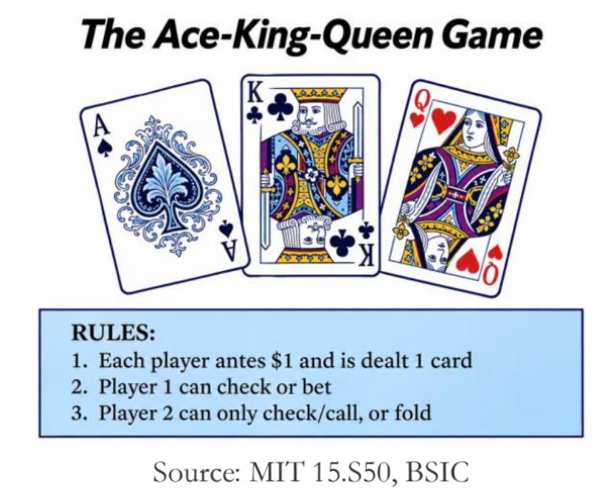
Another example is the Ace-King-Queen Game, a simplified version of poker in which each player receives one card and must decide whether to bet, call, or fold. The game illustrates the indifference principle because the first player must balance value betting with strong hands and bluffing with weak hands, while the second player must choose how often to call. At equilibrium, player 1’s bluffing frequency with the Queen makes player 2 indifferent between calling and folding with the King. Conversely, player 2’s calling frequency with the King makes player 1 indifferent between bluffing and checking with the Queen.
The same logic applies to poker. Consider a simplified final betting round with no raises. The bettor holds either a hand that always wins at showdown or a hand that always loses. The caller holds a “bluff-catcher”: a hand that beats the bettor’s bluffs but loses to their value bets. When the equilibrium involves both bluffing and calling with positive probability, two indifference conditions determine the balance.
- The bettor’s bluffing frequency makes the caller indifferent between calling and folding. Bluff too rarely and calling loses money relative to folding. Bluff too often and calling becomes profitable.
- The caller’s calling frequency makes the bettor indifferent between bluffing and checking with the weak hand. Call too rarely and bluffing becomes profitable relative to giving up. Call too often and bluffing loses money.
These conditions work together. A caller who always folds invites more bluffs; a bettor who never bluffs invites more folds. At equilibrium, neither player can improve their expected payoff by changing these frequencies alone.
Not every hand needs to be indifferent. In this simplified game, value hands bet, while weak hands may mix between bluffing and giving up. More generally, an equilibrium can contain both pure decisions, where one action is always chosen, and mixed decisions, where several actions have equal value.
This also provides intuition for the learning algorithm introduced later. Rather than being given the correct frequencies, it tracks how much better alternative actions would have performed and adjusts play accordingly. In finite two-player zero-sum games with perfect recall, if both players’ average regret approaches zero, their appropriately averaged strategies approach a Nash equilibrium, even if the strategies used in individual iterations keep changing.
We can now write the two indifference conditions in terms of the pot and the bet. The caller’s condition is the break-even condition for a call: it gives the equity needed to call and, equivalently, the share of bets that should be bluffs. The bettor’s condition gives how often the caller must defend. These are the formulas of this simplified model.
The core formulas
Poker players describe stacks, styles and results with a handful of standard statistics. Chips are counted in big blinds (BB), the larger forced bet, so that decisions compare across stake levels. In tournaments, Harrington’s M is the stack divided by the total cost of the blinds and antes over one orbit: roughly how many rounds a player can survive without playing a hand.
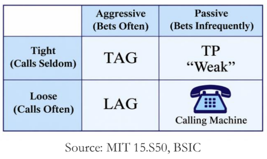
Playing style is summarised by VPIP, the share of hands in which a player voluntarily puts money in before the flop, and PFR, the share in which they raise. A low VPIP marks a tight player and a high one a loose player; a PFR close to VPIP marks an aggressive player, who bets and raises rather than calls. Results are measured in big blinds won per 100 hands, where about 5 BB/100 is a strong online win rate; research uses milli-big-blinds per hand, so 5 BB/100 equals 50 mbb per hand. These statistics describe how someone plays. The formulas below ask how one should play.
The pot contains P before the bet, the bettor wagers B, and we write s = B / P for the bet as a fraction of the pot: s = ½ for a half-pot bet, s = 1 for a pot-sized bet.
The caller’s condition: pot odds and the bluff share. A call costs B. If the bettor is bluffing, the caller wins the pot plus the bet, P + B; if the bettor has a value hand, the call loses B. Suppose that, given the caller’s cards and the betting history, a share x of the bettor’s possible betting hands are bluffs. Calling with a bluff-catcher is then worth x(P + B) − (1 − x)B, while folding is worth zero. The caller is indifferent when:
x=BP+2B=s1+2s
This single number has two readings. From the caller’s perspective, this is the break-even equity implied by the pot odds, since the caller risks B to win P + B. It is the break-even point of the expected-value expression used in our previous article, written here with P as the pot before the bet. From the bettor’s side it is the balanced bluff share: the fraction of bets that should be bluffs so that the caller gains nothing by calling or folding. Equivalently, the betting range should contain s / (1 + s) bluffs for every value bet, counting how often each hand bets, not only which hands can bet.
The bettor’s condition: the defence frequency. A bluff wins the pot P if the caller folds and loses B if called. If the caller folds with probability f, bluffing is worth fP − (1 − f)B, against zero for giving up. The bettor is indifferent when f = B / (P + B), which means the caller must continue with probability:
MDF=PP+B=11+s
This is the minimum defence frequency. If the caller folds more often than 1 − MDF, every bluff becomes profitable; defending at least this often prevents a zero-equity bluff from earning a positive expected payoff.
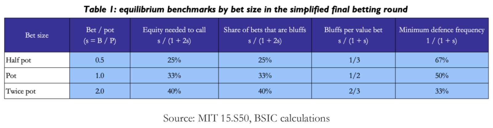
The table shows a counter-intuitive pattern. Larger bets support a higher proportion of bluffs in the betting range. The reason comes from the caller’s decision: a larger bet requires more equity to call, so a balanced betting range can contain more bluffs per value bet while still leaving the bluff-catcher indifferent. Meanwhile, each bluff risks more to win the same existing pot, so the caller can fold more often without making bluffing profitable. These conditions link a chosen bet size to the frequencies that balance it; they do not, by themselves, identify the optimal size.
Our previous article evaluated candidate sizes using estimated opponent responses. Here we derive the frequencies that make a given size balanced in a simplified game. Choosing between sizes requires a further comparison of their strategic consequences.
The pot-odds rule appears in the MIT 15.S50 Basic Strategy lecture, and the calling frequency and bluff-to-value ratio in Matt Hawrilenko’s Game Theory for Humans lecture. All three hold exactly in this simplified model, where hands either always win or always lose and there are no raises or later betting rounds. Real poker relaxes each of these assumptions, and one more matters immediately: card removal.
Card removal affects both sides of the calculation. The caller evaluates the bluff share among betting hands compatible with their own cards. The bettor evaluates the fold frequency among opponent hands compatible with the hand being used to bluff. These conditional frequencies need not equal the corresponding averages across all hands. The next section makes that distinction concrete in a three-card game.
The AKQ game
These ideas are illustrated with the AKQ game, small enough to solve completely. The deck has three cards: Ace, King and Queen. Each player antes one chip and receives one card. Player 1 may check, which goes straight to showdown, or bet one chip; player 2 then calls or folds. The pot before the bet is P = 2 and the bet is B = 1, so s = ½.
The equilibrium uses each type of decision from the previous sections. Player 1 always bets the Ace, checks the King and bluffs with the Queen one third of the time. Betting the King achieves nothing against the Queen, which folds, and loses an additional chip against the Ace, which calls, so checking is better. Player 2 always calls with the Ace, folds the Queen and calls with the King one third of the time. Only the Queen bluff and the King call are mixed, and each is balanced by the opponent’s indifference.
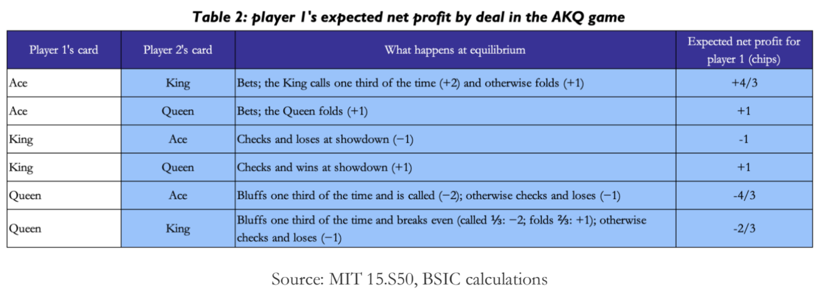
Card removal is what makes these numbers line up with the general formulas. Before player 1 acts, player 2 holding the King thinks the Ace and the Queen are equally likely. Once player 1 bets, that changes. The Ace always bets but the Queen bets only one third of the time, so three bets in four come from the Ace and one in four from the Queen. That makes exactly a quarter of player 1’s bets bluffs. A quarter is also the equity the King needs to call a half-pot bet, so the King is indifferent between calling and folding.
Now look at it from the bluffing Queen’s side. Player 2 holds the Ace or the King with equal probability. The Ace always calls and the King calls one third of the time, so the bluff gets called two thirds of the time, which is the minimum defence frequency for a half-pot bet. Both match the half-pot row of Table 1, but only when measured against the hands each player can actually face. Table 2 shows what the equilibrium is worth to player 1 in each of the six possible deals. All six are equally likely, so player 1’s expected profit per hand is their simple average, 1/18 of a chip. This is the value of the game: no strategy player 2 can choose holds player 1 below it, and no strategy player 1 can choose pushes it higher.
One extra option changes the result
Kuhn poker keeps the three-card deck and the antes, but player 2 is allowed to bet after player 1 checks. Player 1 then has a decision to call or fold. That extra branch changes the incentives: checking can no longer guarantee an immediate showdown.
The equilibrium value for the first player becomes −1/18 of a chip per hand. Kuhn poker also has a family of equilibrium strategies rather than one unique set of frequencies. This makes it a useful test of an algorithm: we can check the value it discovers without expecting every run to return exactly the same mix of actions.
How a computer finds an equilibrium
For AKQ and Kuhn poker we can work through the incentives by hand. For a larger game we need a way to adjust thousands or millions of decisions without solving a separate set of equations at every point. Counterfactual Regret Minimisation, usually shortened to CFR, is one of the standard approaches (Zinkevich et al., 2007).
The idea starts with regret. Suppose we repeatedly make a decision and afterwards compare the payoff of the action we chose with what we would have received by choosing another action. The difference tells us how much we have missed out on. CFR extends this comparison to the information sets of a poker game: the situations a player can distinguish given their own cards and the public history, without knowing the opponent’s cards.
At each iteration, the algorithm walks through the game and estimates the value of the available actions. It accumulates positive regret for actions that would have done better, then uses those regrets to assign probabilities in the next iteration. Actions with more positive regret become more likely. Crucially, the algorithm also tracks the average strategy over the iterations, rather than treating the final iteration as the answer.
In a two-player zero-sum game, as average regret falls, the average strategy profile approaches a Nash equilibrium. CFR does not start with the correct bluffing or calling frequencies. It reaches them by repeatedly comparing what each action would have been worth. That is why recovering −1/18 in Kuhn poker is a meaningful test: the program finds a value we already know from the theory.
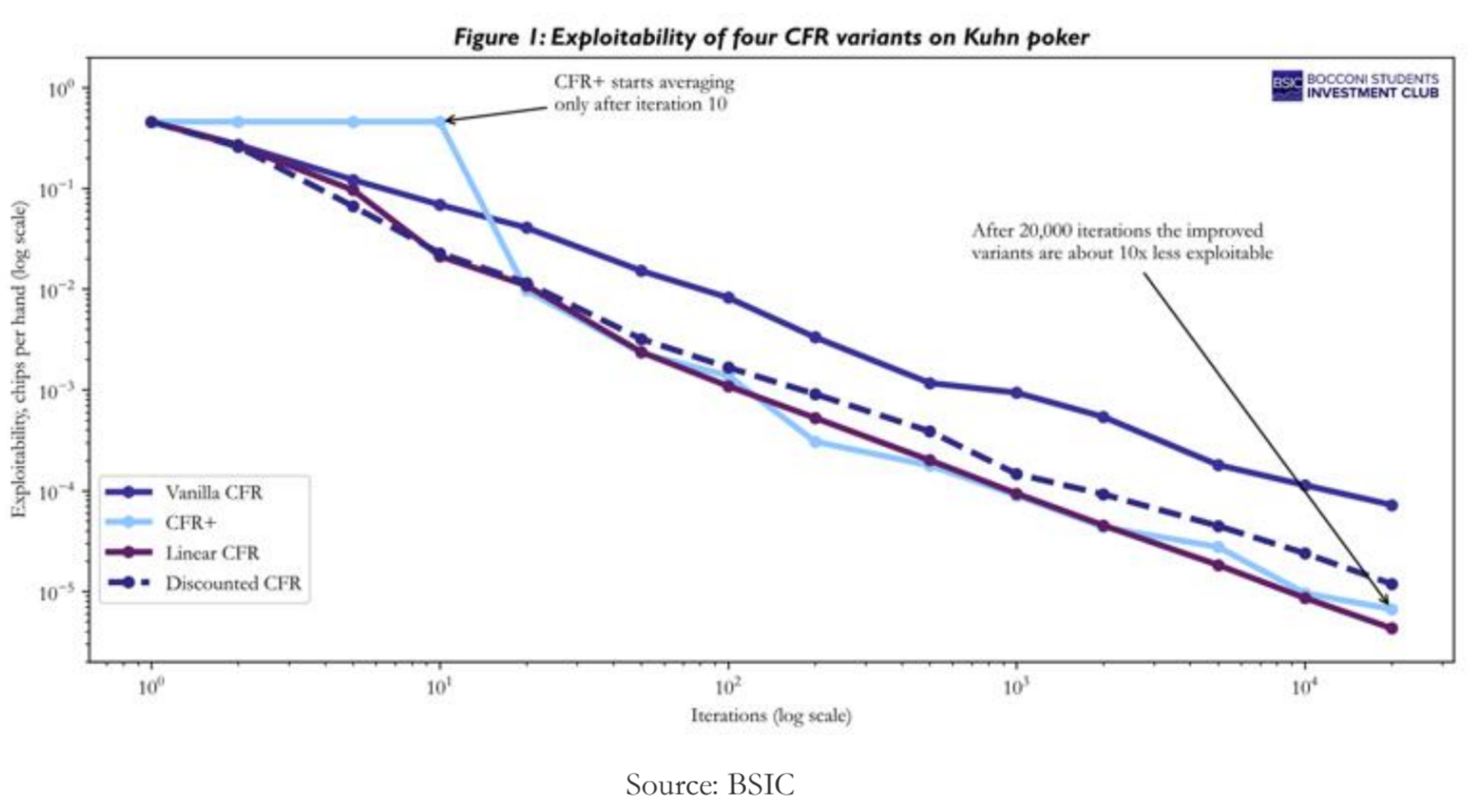
Figure 1 shows our implementation on Kuhn poker. All four variants converge, but at different speeds: after 20,000 iterations the original CFR is still about six to seventeen times more exploitable than the improved variants. On a game this small the difference costs milliseconds; on the hold’em blueprint, where every iteration is expensive, it decides whether training takes days or weeks.
Variants such as CFR+ and discounted CFR change how regrets are accumulated or weighted, often improving practical convergence. They do not remove the underlying problem of game size, however. Full no-limit hold’em is still far beyond what we can solve by directly enumerating every possible decision.
From equilibrium formulas to bot architecture
CFR gives us a way to learn equilibrium-like strategies, but a full no-limit hold’em game remains too large to solve as one enormous tree. There are 1,326 distinct two-card starting combinations, four betting rounds and a huge number of legal betting sequences. The solution is to simplify some decisions in advance and calculate more carefully when a particular hand is actually being played.
Our bot is designed for six-handed no-limit hold’em, with a heads-up solver at its core. This follows both from the mathematical guarantees and from how poker hands develop. Two-player zero-sum games let us measure exploitability; six-player games do not have the same simple minimax protection. And even at a six-handed table, many postflop pots are contested by just two players. The heads-up solver therefore remains useful throughout the larger system.
The architecture
The design draws on DeepStack (Moravčík et al., 2017) for heads-up play and Pluribus (Brown and Sandholm, 2019) for multiplayer play. Both systems combine calculations performed before the hand with further search during play, rather than storing a complete strategy for every possible situation.
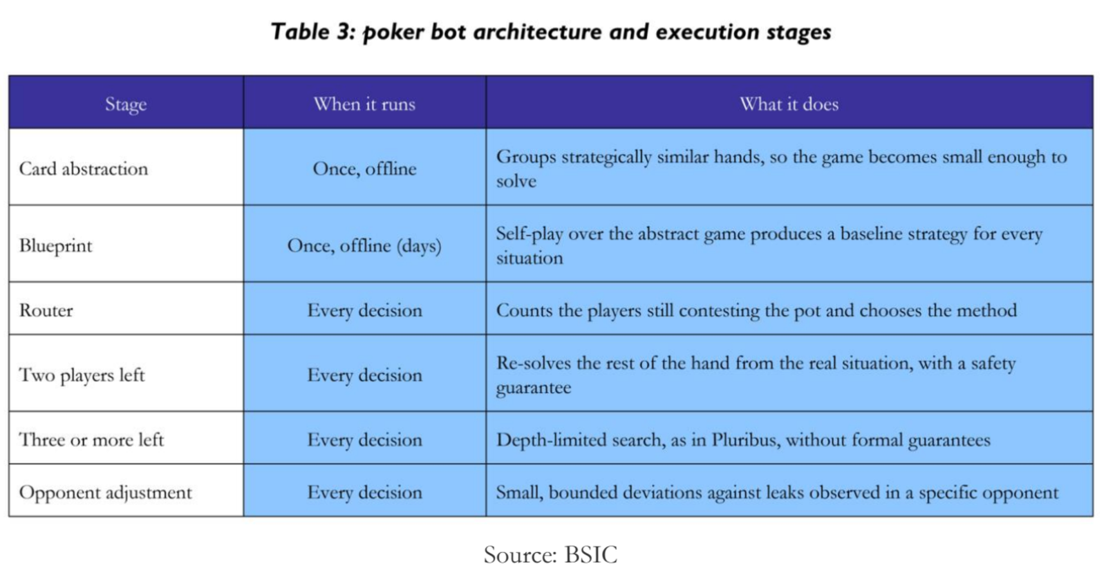
Offline, card abstraction groups strategically similar hands so the blueprint can be trained on a smaller version of the game. The blueprint is a baseline strategy produced through self-play. During a hand, the router checks how many players are still contesting the pot and sends the decision to the appropriate branch. The heads-up branch re-solves the current situation; the multiplayer branch uses depth-limited search. Any opponent-specific adjustment is kept bounded rather than being allowed to replace the baseline freely.
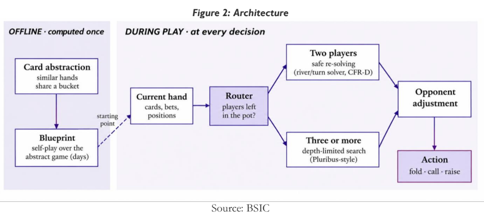
There is an important distinction between designing these components and verifying that they work together as a complete competitive bot. The numerical tests below validate particular engines and solvers; they are not yet a measurement of end-to-end six-handed performance.
Why safe re-solving matters
Re-solving sounds straightforward: take the current turn or river situation and compute a better strategy. The danger is that a locally attractive answer may not be consistent with how the bot played earlier in the hand. If an opponent changes which hands reach that point, they may exploit the mismatch.
CFR-D (Burch, Johanson and Bowling, 2014) deals with this through a constraint on the opponent’s value. Before entering the re-solved part of the game, the opponent has an alternative for each possible hand: take the counterfactual value that hand was allowed under the original strategy. The new strategy must respect those bounds. Under the method’s assumptions, this lets us re-solve without increasing the original strategy’s exploitability.
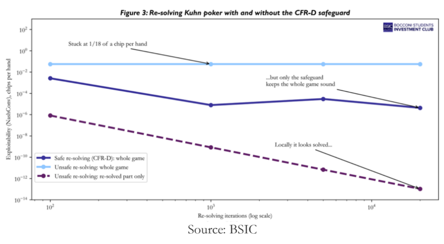
We tested this directly. Starting from an equilibrium strategy for Kuhn poker, we re-solved part of the game with and without the CFR-D safeguard. Without it, the re-solved part looks perfect: its own gap falls to around 10⁻¹³. Yet the full game becomes exploitable by 1/18 of a chip per hand, because the new strategy no longer fits with how the hand was played before. With the safeguard, exploitability of the whole game stays close to zero.
The same formal guarantee does not extend directly to a game with three or more active players. For those situations, the bot uses depth-limited search, and we must judge the quality of its decisions through experiments rather than a minimax bound.
How we test it
Before asking whether a bot plays well, we need to check that it is playing the right game. A side pot paid to the wrong player or an illegal re-raise accepted after a short all-in can quietly corrupt training without ever crashing the program. That is why we first test the rules and hand evaluation, then the solving algorithms.
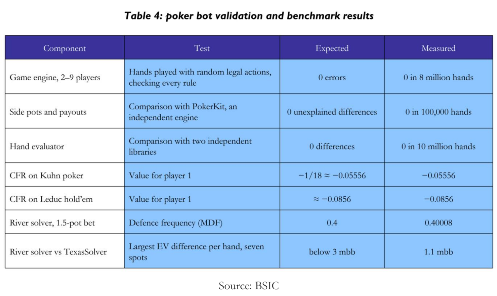
The first three comparisons check the engine rather than the strategy. We ran eight million hands with random legal actions, compared 100,000 hands with PokerKit and tested ten million hand evaluations against two independent libraries. None produced an unexplained difference. These tests do not prove that the engine is free of bugs, but they reduce the risk of training on incorrect rules.
The algorithm tests take us back to the earlier examples. Our CFR implementation recovered the Kuhn poker equilibrium value of −1/18, approximately −0.05556, from the rules and payoffs alone. We then tested Leduc hold’em, a somewhat larger benchmark game, and obtained the expected value of approximately −0.0856.
The river solver was also checked against the simple defence-frequency calculation. For a bet of 1.5 times the pot, the model gives:
MDF=11+1.5=0.4
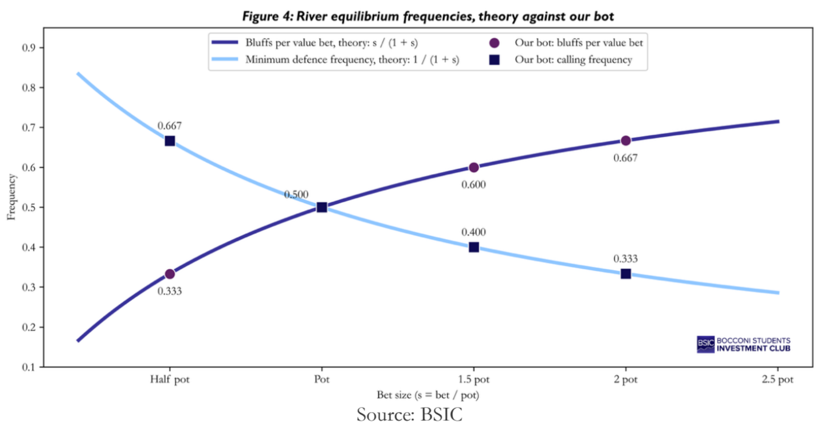
Figure 4 places our bot’s river decisions on the curves from Table 1. The bot was never given the formulas; it found the frequencies from the payoffs alone. Across the four bet sizes, its bluffing and calling frequencies differ from the theoretical values by less than 0.0002.
The measured result was 0.40008. The solver was not given the MDF formula; it reached the frequency from the actions and payoffs of that test game. This is a benchmark for the simplified setting, not a claim that every real river situation must defend exactly 40%.
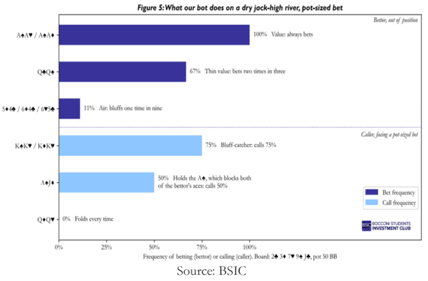
The simplified model has only two kinds of hand. Figure 5 shows the bot on a slightly richer river, where both players hold several hands, including some that block each other. Aces always bet. Queens bet two times in three, as thin value against weaker pairs. The hands with no showdown value bluff only one time in nine: the range is no longer polarised, so the one-bluff-per-two-value-bets rule from Table 1 no longer applies directly. The caller’s choices show card removal at work. Kings, which beat everything except aces, call 75% of the time. Ace-jack is weaker, yet still calls half the time, because its ace of spades makes both of the bettor’s aces impossible. None of these frequencies was programmed; each emerges from the equilibrium computation.
Not every comparison agreed perfectly. Brown and Sandholm’s (2019) discounted-CFR paper gives a deliberately extreme three-action example with payoffs of 0, 1 and −1,000,000. In their account, CFR+ takes 471,407 iterations to stop selecting the worst action, compared with 970 for LCFR. We reproduced 471,407 for CFR+ but obtained 972 for LCFR. We checked the result independently with 60-digit arithmetic and tested plausible weighting conventions without reproducing 970. We report the discrepancy rather than force a match; the large convergence advantage in this example is unchanged.
We also compared our river solver with TexasSolver. The initial results differed substantially because TexasSolver’s reported strategy heavily weighted roughly the final ten iterations. After recalculating its average strategy across all iterations, the solvers agreed closely. Over seven tested situations, the largest expected-value difference was 1.1 milli-big-blinds per hand.
Conclusion
Building a poker bot required translating strategic principles into decisions under imperfect information. Nash equilibrium defined the objective, while counterfactual regret minimisation provided a method for approaching it. The resulting design combined an offline blueprint with search during play, balancing computational constraints with the distinct challenges of heads-up and multiplayer poker.
Our tests provided evidence of the engine’s reliability and the solvers’ accuracy in the settings examined. They recovered known game values, reproduced simplified equilibrium frequencies and showed why locally accurate re-solving can still increase full-game exploitability without appropriate safeguards.
These results were promising: the tested components reproduced theoretical benchmarks and agreed closely with an independent solver on the expected values examined. They provide a foundation for evaluating the complete bot in six-handed hold’em, where competitive performance, computational efficiency and robustness remain to be established.
References
Brown, Noam and Sandholm, Tuomas, “Solving Imperfect-Information Games via Discounted Regret Minimization”, 2019
Brown, Noam and Sandholm, Tuomas, “Superhuman AI for multiplayer poker”, 2019
Burch, Neil, Johanson, Michael and Bowling, Michael, “Solving Imperfect Information Games Using Decomposition”, 2014
Chen, Bill and Ankenman, Jerrod, “The Mathematics of Poker”, 2006
Desmond, Kevin, “Basic Strategy”, lecture in MIT 15.S50 Poker Theory and Analytics, 2015
Harrington, Dan and Robertie, Bill, “Harrington on Hold’em, Volume II: The Endgame”, 2005
Hawrilenko, Matt, “Game Theory for Humans”, lecture in MIT 15.S50 Poker Theory and Analytics, 2015
Kelly, John L., “A New Interpretation of Information Rate”, 1956
Kim, Juho, “PokerKit: A Comprehensive Python Library for Fine-Grained Multi-Variant Poker Game Simulations”, 2023
Kuhn, Harold W., “A Simplified Two-Person Poker”, 1950
Lisý, Viliam and Bowling, Michael, “Equilibrium Approximation Quality of Current No-Limit Poker Bots”, 2017
MIT OpenCourseWare, “15.S50 Poker Theory and Analytics”, 2015
Moravčík, Matej et al., “DeepStack: Expert-Level Artificial Intelligence in Heads-Up No-Limit Poker”, 2017
Nash, John F., “Equilibrium Points in N-Person Games”, 1950
Southey, Finnegan et al., “Bayes’ Bluff: Opponent Modelling in Poker”, 2005
Tammelin, Oskari, “Solving Large Imperfect Information Games Using CFR+”, 2014
von Neumann, John, “Zur Theorie der Gesellschaftsspiele”, 1928
Zinkevich, Martin et al., “Regret Minimization in Games with Incomplete Information”, 2007
Kim, Juho et al., “PokerKit”, GitHub repository, https://github.com/uoftcprg/pokerkit
Lee, Henry, “PokerHandEvaluator”, GitHub repository, https://github.com/HenryRLee/PokerHandEvaluator
Andrews, Julian, “eval7”, GitHub repository, https://github.com/JulianAndrews/pyeval7
bupticybee, “TexasSolver”, GitHub repository, https://github.com/bupticybee/TexasSolver
Brown, Noam, “poker_solver”, open-source river solver, 2025



0 Comments