Trading the Network III: From Predictive Alpha to Tradable Alpha

Introduction

The first two parts of this research separated three questions that are often collapsed into one. The first asked whether a more sophisticated machine-learning architecture necessarily produces better equity forecasts. Ridge regression outperformed the Multilayer Perceptron, Graph Convolutional Network and Graph Attention Network when all models were given the same stock-level information. The second asked whether this failure meant that relationships between securities were useless. Once the graph was changed from contemporaneous similarity to a sparse, directed residual lead-lag network, Graph-Augmented Ridge improved the mean rank Information Coefficient from approximately 0.02893 to 0.03283. The predictive edge existed; conventional message passing was simply not the best way to use it.

That improvement created a new problem. The residual lead-lag Graph Ridge model produced better forecasts than ordinary Ridge, but its portfolio traded more aggressively. At the baseline assumption of ten basis points of transaction cost per unit of turnover, the additional trading absorbed much of the forecasting advantage. Article III therefore leaves the forecasting model unchanged and asks a deliberately narrower question: can the same predictions be converted into positions more efficiently?

A forecasting model and a trading strategy are not the same object. A model produces a score describing expected relative performance. A portfolio rule decides whether that score is sufficiently different from yesterday’s score to justify changing a real position. Every change in holdings incurs a cost. Consequently, a forecast can contain genuine information and still fail as a trading strategy if the portfolio reacts too mechanically to small changes in rank.

The experiment freezes the strongest Part II forecasting specification: Residual Lead-Lag Graph Ridge with one predictive predecessor per stock. No new predictive variables, graph definitions or neural architectures are introduced. We then test a controlled family of portfolio rules designed to reduce unnecessary turnover or improve the relationship between forecast strength, risk and trading intensity. These include wider entry-exit buffers, partial position adjustment, slower rebalancing, inverse-volatility weighting, confidence filtering, a validation-based expected-edge gate and combinations of these mechanisms.

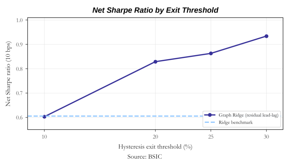
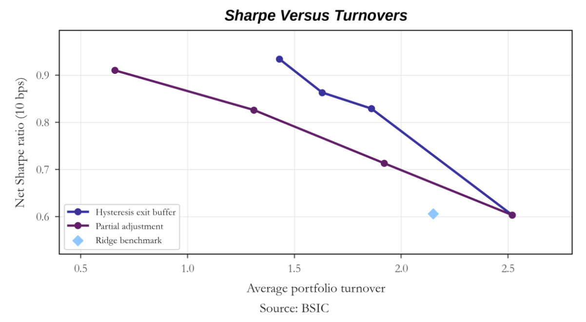
The results are economically meaningful but also restrictive. The baseline Graph Ridge strategy earns approximately 10.14% per year with 19.03% annualised volatility and a Sharpe ratio of 0.603 after ten basis points of assumed transaction cost. The strongest tested implementation is a wide hysteresis rule: stocks enter the long or short portfolio at the original 10% threshold but are not removed until they cross a 30% exit boundary. This raises annualised return to 14.66%, reduces volatility to 16.04%, cuts average turnover from 2.52 to 1.43, and raises the net Sharpe ratio to 0.934. A different mechanism, adjusting only 25% of the desired portfolio change at each rebalance, produces a Sharpe ratio of 0.910 with turnover of only 0.66 and a maximum drawdown of approximately 24.5%.

The central conclusion is therefore that a substantial portion of the economic weakness identified in Part II came from over-trading a slowly varying signal. Portfolio inertia recovers meaningful risk-adjusted performance, but even the strongest tested implementation remains below a net Sharpe ratio of one. The next stage must therefore improve the information content of the edge itself while preserving the turnover discipline learned here.

The Model We Are Trading: Residual Lead-Lag Graph Ridge

Before changing the portfolio construction, it is useful to make precise what the forecasting model actually does. The model used throughout Article III is Residual Lead-Lag Graph Ridge with one predictive predecessor per stock. Despite the name, it is not a Graph Neural Network. It is a regularised linear regression supplied with graph-derived information. Its architecture can be understood as a sequence of four steps: remove common market movements, identify directional lead-lag relationships, construct relative features between each stock and its strongest predecessor, and use Ridge regression to forecast the stock’s future cross-sectional return rank. This is the forecasting specification that Article II found to contain the strongest relational information, and Article III leaves it unchanged.

The first step is residualisation. Two stocks can move together simply because both respond to the market or their common sector. For example, Nvidia and AMD may both rise when the technology sector rallies even if neither contains useful information about the other’s future return. We therefore attempt to remove these broad common movements before constructing the graph. Conceptually, the return of stock $i$ is decomposed as

$r_{i,t} = \alpha_{i} + \beta_{i,M}r_{M,t} + \beta_{i,S}r_{S(i),t} + \varepsilon_{i,t},$

where $r_{M,t}$ is the broad market return, $r_{S(i),t}$ is the return of stock $i$ ’s sector, and $\varepsilon_{i,t}$ is the residual return left after these common exposures have been removed. The residual is therefore intended to capture the more stock-specific component of the movement. This does not make the residual perfectly idiosyncratic or establish causality, but it reduces the chance that the graph merely rediscovers broad market and sector co-movement.

The second step is to search for lead-lag relationships between these residual returns. Ordinary contemporaneous correlation asks whether two stocks tend to move at the same time. A lead-lag relationship instead asks whether movement in one stock tends to occur before movement in another. For a candidate leader $j$ , target stock $i$ , and positive lag $\mathcal{l}$ , we estimate a historical relationship of the form

$\rho_{j \rightarrow i}^{\left( \mathcal{l} \right)} = Corr\left( \varepsilon_{j,t\mathcal{- l}},\varepsilon_{i,t} \right).$

The direction of the arrow is important. A high value means that movements in stock $j$ have historically been associated with movements in stock $i$ occurring $\mathcal{l}$ periods later. The relationship is still statistical rather than causal, but it is much closer to the economic mechanism required for forecasting than simple contemporaneous similarity.

For every target stock $i$ , the model searches the candidate lead-lag relationships using only information available at that historical date and retains the single strongest predictive predecessor. If that stock is denoted $j^{*}(i,t)$ , then

$j^{*}(i,t) = \underset{j}{arg\, max}\mspace{6mu}\rho_{j \rightarrow i,t}^{\left( \mathcal{l}^{*} \right)}.$

The notation $arg\, max$ simply means “choose the stock associated with the largest estimated relationship.” Setting

$k = 1$

means that each target receives graph information from only one predecessor rather than averaging information across many neighbours. Article II found this extreme sparsity to be important: adding three or five neighbours diluted rather than strengthened the predictive signal.

The third step converts this edge into variables that a forecasting model can actually use. Let

$X_{i,t}$

denote the target stock’s own feature vector, containing the same stock-level characteristics used throughout the research, such as recent returns, volatility, liquidity and market beta. Let

$N_{i,t} = X_{j^{*}(i,t),t}$

denote the corresponding feature vector of its strongest predictive predecessor. The model then explicitly constructs the network dislocation

$D_{i,t} = X_{i,t} - N_{i,t}.$

This third object is crucial. Suppose the predecessor has very strong five-day momentum while the target stock has barely moved. The potentially useful information may not be the leader’s momentum or the lagger’s momentum independently, but the fact that a historically predictive leader has moved while the target has not. The difference $D_{i,t}$ gives the model direct access to precisely this relative state.

The complete Graph Ridge input is therefore the concatenated vector

$Z_{i,t} = \begin{bmatrix} X_{i,t} \\ N_{i,t} \\ D_{i,t} \end{bmatrix} = \begin{bmatrix} \text{Own Features} \\ \text{Leader Features} \\ \text{Own Features} - \text{Leader Features} \end{bmatrix}.$

This architecture is deliberately different from conventional GNN message passing. A GCN would partially mix the target and neighbour representations into a new representation. Graph Ridge keeps all three pieces separate. It can therefore learn that the target’s own momentum matters positively, the leader’s momentum matters differently, and the gap between the two contains additional information. Nothing forces these quantities to be averaged together.

Finally, Ridge regression maps these graph-augmented features into the predicted future rank:

${\widehat{y}}_{i,t} = \beta_{0} + \beta_{X}^{\top}X_{i,t} + \beta_{N}^{\top}N_{i,t} + \beta_{D}^{\top}D_{i,t}.$

The three coefficient vectors have distinct interpretations. $\beta_{X}$ determines how the target stock’s own characteristics affect its forecast; $\beta_{N}$ determines how the predecessor’s characteristics affect it; and $\beta_{D}$ determines whether the difference between the target and its predecessor contains additional predictive information.

The parameters are estimated using the Ridge objective

$\widehat{\beta} = \underset{\beta}{arg\, min}\left\lbrack \sum_{i,t}^{}\left( y_{i,t} - Z_{i,t}^{\top}\beta \right)^{2} + \lambda \parallel \beta \parallel_{2}^{2} \right\rbrack.$

The first term asks the model to minimise historical forecasting errors. The second penalises unnecessarily large coefficients and therefore reduces the tendency of the regression to react excessively to noise. This regularisation is especially important because financial return predictability is weak and the graph-derived variables are correlated with the stock’s own characteristics.

The final output is ${\widehat{y}}_{i,t}$ , which is not a predicted percentage return. It is the model’s estimate of where stock $i$ should rank within the subsequent five-day cross-section. A high score identifies a predicted relative winner and a low score a predicted relative loser. The portfolio layer studied in Article III then decides how aggressively those scores should be converted into actual positions.

The economic hypothesis is equally simple. Markets may not incorporate information everywhere simultaneously. If one security historically tends to move before another, an unusual state in the leader combined with a remaining dislocation in the lagger may contain information about which security will subsequently outperform. Residualisation attempts to isolate this relationship from common market movements, the lead-lag graph supplies direction, $k = 1$ prevents weak neighbours from diluting the strongest relationship, the dislocation features preserve relative information, and Ridge provides a deliberately conservative way of translating that information into a forecast.

This is precisely why Article III freezes the model. Its purpose is no longer to determine whether the forecasting architecture contains information: Article II already established that the residual lead-lag Graph Ridge improves the forecasting statistics relative to ordinary Ridge. Article III instead takes the resulting ${\widehat{y}}_{i,t}$ as given and asks whether the portfolio should react to every movement in that forecast.

From a Forecast to a Portfolio

A cross-sectional forecasting model produces one predicted score for every eligible stock at each signal date. Denote this score by

${\widehat{y}}_{i,t}.$

The score is a forecast of the stock’s relative position in the subsequent five-day return distribution. A high value means that the model expects stock $i$ to outperform a large part of the contemporary cross-section; a low value means that it expects the stock to underperform.

The simplest portfolio rule ranks all stocks by ${\widehat{y}}_{i,t}$ and buys the top 10% while shorting the bottom 10%. Let $L_{t}$ denote the long set and $S_{t}$ the short set. Under equal weighting, the target weight of stock $i$ is approximately

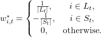
$w_{i,t}^{*} = \left\{ \begin{matrix} \frac{1}{\left| L_{t} \right|}, & i \in L_{t}, \\ - \frac{1}{\left| S_{t} \right|}, & i \in S_{t}, \\ 0, & \text{otherwise}. \end{matrix} \right.$

The long side therefore has gross exposure of approximately $+ 1$ , the short side approximately $- 1$ , and the complete portfolio has gross exposure near two and net exposure near zero:

$\sum_{i}^{}\left| w_{i,t} \right| \approx 2,\quad\quad\sum_{i}^{}w_{i,t} \approx 0.$

This is attractive as an experimental benchmark because it translates model rankings into positions without introducing a separate optimisation model. It is also mechanically aggressive. If a stock ranked at the 9.9th percentile one week and the 10.1th percentile the next, it can move from fully invested to zero even though the underlying forecast has barely changed. Another stock then enters to replace it. The ranking signal has moved slightly, but the portfolio has made two trades.

The distinction between a target portfolio and an implemented portfolio is therefore central to Article III. The target portfolio, $w_{t}^{*}$ , is what the latest forecast would hold if trading were free. The implemented portfolio, $w_{t}$ , is what an investor actually chooses to hold after considering the cost of moving from the previous position. Article III studies alternative mappings

$\left( {\widehat{y}}_{t},w_{t - 1} \right) \rightarrow w_{t}$

while keeping ${\widehat{y}}_{t}$ fixed.

Why Turnover Matters

Turnover measures how much the portfolio changes between two rebalancing dates. In the backtest it is defined as

$TO_{t} = \sum_{i}^{}\left| w_{i,t} - w_{i,t - 1} \right|.$

Suppose a portfolio sells a 1% position in one stock and buys a 1% position in another. The absolute weight change is 1% on the sale and 1% on the purchase, so the total turnover contribution is 2%. This convention captures both sides of the rebalance.

Transaction costs are then applied proportionally to turnover. If $c$ denotes the assumed cost per unit of turnover, net portfolio return is

$r_{p,t}^{net} = r_{p,t}^{gross} - c\, TO_{t}.$

At ten basis points,

$c = 0.001.$

A weekly turnover of $TO_{t} = 2$ therefore creates an approximate cost of $0.2\%$ for that rebalance. Repeated across the year, small costs can become economically large. This is exactly what happened to the Part II Graph Ridge strategy: it possessed stronger predictive information than ordinary Ridge but changed its rankings sufficiently often that the portfolio paid more to exploit them.

The annual cost drag reported in Article III is the annualised effect of this turnover-based cost term. The baseline Graph Ridge portfolio has average turnover of approximately 2.52 and annual cost drag of approximately 13.10 percentage points under the ten-basis-point assumption.

A useful complementary statistic is the break-even transaction cost. This asks how high costs could rise before the strategy’s estimated net economic advantage is exhausted. A strategy that works only at one or two basis points is much more fragile than one that remains profitable at twenty or thirty basis points. The baseline Graph Ridge break-even cost is approximately 17.4 basis points. Several turnover-aware implementations raise this materially.

Measuring Portfolio Performance

The primary economic statistic is the Sharpe ratio. Let ${\bar{r}}_{w}$ denote the average weekly portfolio return and $\sigma_{w}$ its weekly standard deviation. Ignoring a small weekly risk-free rate for this comparative experiment, the annualised Sharpe ratio is approximately

$SR = \frac{{\bar{r}}_{w}}{\sigma_{w}}\sqrt{52}.$

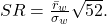
The numerator rewards return while the denominator penalises variability. A strategy earning 15% with 10% volatility is economically different from one earning the same 15% with 30% volatility, even though their raw returns are identical.

Annualised volatility is computed from weekly return variation as

$\sigma_{ann} = \sigma_{w}\sqrt{52}.$

Annualised return is obtained from the compounded weekly wealth process. If $r_{p,t}$ is the weekly net return, cumulative wealth evolves according to

$W_{T} = \prod_{t = 1}^{T}\left( 1 + r_{p,t} \right),$

and the annualised return rescales the resulting growth rate to a one-year horizon.

Maximum drawdown measures the largest peak-to-trough decline in cumulative wealth. If $W_{t}$ is the wealth index and $M_{t} = \max_{s \leq t}W_{s}$ is the previous running maximum, drawdown is

$DD_{t} = \frac{W_{t}}{M_{t}} - 1,$

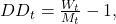
and maximum drawdown is the minimum value of $DD_{t}$ over the sample. Drawdown matters because two strategies with similar Sharpe ratios can impose very different capital and behavioural burdens on an investor.

Finally, the hit rate reports the fraction of weekly observations with positive net return. It is not a substitute for Sharpe—many profitable strategies win less than half the time but have larger gains than losses—but it provides an intuitive description of return consistency.

Experiment 1: Hysteresis and Rank Buffers

The first intervention addresses a simple source of turnover: stocks repeatedly crossing a sharp portfolio boundary. Under the baseline rule, a stock enters the long portfolio when it lies in the top 10% and exits as soon as it falls outside that same top 10%. Entry and exit therefore occur at the identical threshold.

Hysteresis separates these decisions. A stock still needs a strong signal to enter, but once held it is allowed to remain in the portfolio until its signal deteriorates substantially. If $q_{i,t}$ denotes the cross-sectional percentile of the prediction score, a simplified long-side rule is

$\text{Enter long if }q_{i,t} \geq 1 - q_{entry},$

but

$\text{Exit long only if }q_{i,t} < 1 - q_{exit},$

where $q_{exit} > q_{entry}$ . The short side is symmetric.

With $q_{entry} = 0.10$ and $q_{exit} = 0.20$ , for example, a stock must enter in the top 10% but can remain long while it stays within the top 20%. This creates a buffer around the trading boundary. Small rank fluctuations no longer force immediate transactions.

The economic intuition is that forecasts are noisy estimates, not exact state variables. A stock moving from the 9th to the 11th percentile has not necessarily experienced a meaningful deterioration in expected return. Treating that tiny rank movement as a command to liquidate assumes a level of forecast precision that the model does not possess. Hysteresis acknowledges estimation error by requiring stronger evidence to reverse an existing decision than to maintain it.

The results strongly support this mechanism. At a 20% exit threshold, Graph Ridge Sharpe rises from 0.603 to 0.829 while average turnover falls from 2.52 to 1.86. Widening the buffer to 25% raises Sharpe further to 0.863 and lowers turnover to 1.63. The strongest tested hysteresis specification uses a 30% exit threshold. It earns approximately 14.66% annually with 16.04% volatility, a Sharpe ratio of 0.934, maximum drawdown of -31.35%, and turnover of only 1.43.

The progression is important:

$SR_{10\%} = 0.603,\quad\quad SR_{20\%} = 0.829,\quad\quad SR_{25\%} = 0.863,\quad\quad SR_{30\%} = 0.934.$

At the same time,

$TO_{10\%} = 2.52 \rightarrow TO_{30\%} = 1.43.$

The Sharpe improvement is therefore accompanied by precisely the mechanism hypothesised in advance: lower turnover and greater portfolio persistence.

Why Hysteresis Can Improve More Than Costs Alone

It would be tempting to interpret the hysteresis result as merely saving transaction costs. The evidence suggests something stronger. The baseline Graph Ridge strategy at zero assumed transaction cost has a Sharpe ratio of roughly 1.28 in Part II. In Article III, the 30% hysteresis strategy has a zero-cost Sharpe of approximately 1.397. Hysteresis therefore improves the gross risk-adjusted return as well as the net result.

This can occur because excessive rank switching is not merely expensive; it can also replace useful positions with noisy marginal alternatives. If the underlying alpha is persistent, yesterday’s high-conviction stock may remain attractive even after slipping slightly in the cross-sectional ranking. A strict weekly re-sort discards that information about position history. Hysteresis implicitly adds a small amount of temporal memory to the portfolio rule.

The result can be understood as a form of decision smoothing. The forecasting model remains responsive, but the portfolio requires a larger state change before acting. This is economically analogous to distinguishing a change in an estimate from a change large enough to justify a transaction.

Experiment 2: Partial Position Adjustment

The second intervention changes how quickly the current portfolio moves toward it. Let $w_{t - 1}$ denote current holdings and $w_{t}^{*}$ the new target portfolio implied by the latest forecast. Full rebalancing sets

$w_{t} = w_{t}^{*}.$

Partial adjustment instead uses

$w_{t} = (1 - \gamma)w_{t - 1} + \gamma w_{t}^{*},$

where

$0 < \gamma \leq 1.$

If $\gamma = 1$ , the strategy is the original full rebalance. If $\gamma = 0.5$ , only half of the desired change is executed at the current rebalance. If $\gamma = 0.25$ , only one quarter is executed.

For example, suppose a stock currently has weight 0 and the new target weight is 2%. Under full adjustment, the portfolio immediately buys 2%. Under $\gamma = 0.25$ , the first adjustment buys only 0.5%. If the target remains 2% the following week, the next position becomes

$0.75(0.5\%) + 0.25(2\%) = 0.875\%.$

The position approaches the target gradually rather than jumping to it.

Partial adjustment is economically sensible when the signal is persistent but noisy. If a forecast reverses one week later, the portfolio has avoided paying the full cost of a position that existed only briefly. The price paid for this stability is slower reaction to genuinely new information.

The experiment reveals a clear trade-off. Full adjustment reproduces the baseline Graph Ridge Sharpe of 0.603 and turnover of 2.52. A 75% adjustment raises Sharpe to 0.713 and lowers turnover to 1.92. A 50% adjustment produces Sharpe 0.826 with turnover 1.31. The strongest tested value is $\gamma = 0.25$ , which produces annualised return of approximately 11.14%, volatility of 12.47%, Sharpe of 0.910 and maximum drawdown of only -24.50%. Average turnover falls dramatically to 0.66.

The relationship is again economically coherent:

$\gamma \downarrow \quad \Rightarrow \quad TO \downarrow ,$

while Sharpe initially rises because the reduction in volatility and trading noise more than compensates for slower response.

The partial-adjustment strategy also has the highest tested break-even cost among the Graph Ridge sensitivity variants, approximately 40.6 basis points. This does not mean that the strategy would necessarily remain attractive under a realistic 40-basis-point implementation environment; rather, it shows that its low turnover makes its economics substantially less fragile to proportional trading costs.

Experiment 3: Changing Portfolio Breadth

Another natural question is whether the original top/bottom 10% portfolio is too broad or too narrow. A smaller tail concentrates capital in the strongest forecasts but may increase volatility and turnover. A broader tail diversifies more heavily but includes weaker signals.

The experiment therefore varies the entry quantile. A 5% portfolio trades only the most extreme predictions. At ten basis points it raises annualised Graph Ridge return to approximately 15.36%, but volatility rises to 23.56% and Sharpe reaches only 0.725. A 15% portfolio reduces volatility to approximately 16.70% but also dilutes expected return, producing Sharpe around 0.648. The original 10% breadth remains between these extremes.

The result suggests that the central Article III problem is not solved simply by concentrating on fewer names. Stronger tails raise raw return but do not create the same risk-adjusted improvement as introducing portfolio persistence.

Experiment 4: Slower Rebalancing

A straightforward way to reduce turnover is to rebalance less frequently. If the baseline strategy rebalances every week, a biweekly strategy can only change positions every second signal date. This mechanically lowers trading activity.

The result, however, is negative. Graph Ridge turnover falls from approximately 2.52 to 1.37, but annualised return falls to 6.48% and Sharpe to 0.460. Simply waiting longer is therefore not equivalent to intelligently retaining positions.

This distinction is important. Hysteresis and partial adjustment still observe every new forecast. They merely require more evidence or more time before fully changing the position. A biweekly rule ignores every second opportunity to react. If genuinely informative shocks occur between scheduled rebalances, the strategy cannot respond.

The experiment therefore separates portfolio inertia from information neglect. The former helps; the latter does not.

Experiment 5: Inverse-Volatility Weighting

Equal weighting assigns the same absolute weight to every selected security. Yet selected stocks can have very different levels of realised risk. A common portfolio construction alternative is inverse-volatility weighting, under which the raw position size is proportional to

${\widetilde{w}}_{i,t} \propto \frac{1}{\sigma_{i,t}}.$

The weights are then rescaled so that the long and short books retain the intended gross exposure. The intuition is that a high-volatility stock should receive a smaller capital weight than a low-volatility stock if the objective is to distribute risk more evenly.

Applied directly to the baseline Graph Ridge portfolio, inverse-volatility weighting does not materially improve performance. Annualised volatility falls from 19.03% to 17.95%, but annualised return also falls, leaving Sharpe almost unchanged at approximately 0.601. Turnover actually rises to 2.69 because changing volatility estimates create an additional source of weight movement.

Combining inverse-volatility weighting with hysteresis performs better, producing annualised return of approximately 13.04%, volatility of 16.55% and Sharpe of 0.824. This is useful, but still weaker than simple wide hysteresis. The conclusion is therefore that risk weighting is not the primary missing ingredient in this signal.

Experiment 6: Confidence Filtering

A natural response to weak financial forecasts is to trade only when the model appears unusually confident. Article III therefore tests a simple confidence filter based on the extremity of prediction scores. The idea is that observations near the centre of the predictive distribution may contain too little expected edge to justify trading.

In the tested implementation, however, a one-standardised-unit confidence filter changes almost nothing. Graph Ridge annualised return remains approximately 10.11%, volatility 19.03%, Sharpe 0.601 and turnover 2.52. The average number of long and short positions is also almost unchanged.

This is an informative negative result. A confidence rule is useful only if its confidence measure actually distinguishes high-quality forecasts from low-quality forecasts. Simply thresholding the magnitude of the existing score does not create that distinction here. Article IV should therefore treat confidence as something that must be modelled from edge quality, persistence or forecast uncertainty, rather than assumed to be synonymous with score extremity.

Experiment 7: Expected Edge Versus Trading Cost

The most economically ambitious portfolio rule asks whether the expected incremental return from a trade is large enough to compensate for its expected cost. In principle, a rational trading rule should execute only when

${\widehat{\alpha}}_{i,t} > {\widehat{Cost}}_{i,t} + m,$

where ${\widehat{\alpha}}_{i,t}$ is estimated expected alpha and $m$ is a safety margin for estimation error.

To avoid using future test information, the Article III implementation estimates the mapping from model score to realised relative return using the preceding validation period only. That historical mapping is then applied to the unseen test period. The design is therefore chronologically valid: the test year’s realised returns never determine whether a contemporaneous test trade is permitted.

Despite its appealing economic logic, the expected-edge gate performs poorly. At a ten-basis-point threshold, Graph Ridge annualised return falls to approximately 8.19%, volatility rises to 24.17%, Sharpe falls to 0.447 and turnover rises to 2.70. The gate also reduces the average number of long and short names substantially.

Why can an apparently rational filter make the strategy worse? Because the estimated mapping from score to expected return is itself noisy and unstable. The procedure introduces a second forecasting problem on top of the first: it must estimate not only which stocks will outperform, but also the magnitude of that expected advantage sufficiently accurately to compare it with costs. The original model was deliberately designed as a ranking model, not a well-calibrated expected-return model. Asking it to support a precise expected-dollar-edge decision can therefore impose more estimation error than it removes.

This failure provides an important lesson for later articles: economic sophistication is useful only when the required quantity can be estimated reliably.

Combining Turnover Controls

Article III also tests whether individually sensible mechanisms reinforce one another. A combination of 20% hysteresis and 50% partial adjustment produces annualised return of approximately 10.49%, volatility of 12.58%, Sharpe 0.857, maximum drawdown -28.13% and turnover 1.06. A broader pre-specified combination adding inverse-volatility weighting, a mild confidence threshold and a small expected-edge gate produces Sharpe 0.844 with volatility 12.37% and turnover 1.12.

These combinations substantially reduce risk and drawdown, but neither beats the best single wide-hysteresis rule on Sharpe. This is another useful result. Portfolio mechanisms are not independent sources of alpha. Combining several conservative rules can over-dampen the signal. The objective is not to minimise turnover at any cost; it is to minimise unproductive turnover while retaining responsiveness to genuine information.

Main Results

The principal portfolio results at ten basis points per unit of turnover are summarised by the comparisons below. Figure 1 isolates how wider hysteresis exit thresholds affect net Sharpe.

The most important pattern is not simply the maximum Sharpe. It is the shape of the results. The interventions that explicitly preserve existing positions like hysteresis and partial adjustment worked. Interventions that merely traded less often, changed risk weights or imposed an additional noisy forecast did not.

The Sharpe-turnover relationship makes the same point visually. The best Graph Ridge implementations move northwest relative to the baseline: they achieve higher Sharpe with lower turnover.

Transaction-Cost Sensitivity

A portfolio construction improvement is much more convincing if it survives a range of transaction-cost assumptions. For the strongest 30% hysteresis strategy, the zero-cost annualised return is approximately 23.50% and Sharpe 1.397. At five basis points, return is 19.00% and Sharpe 1.166. At ten basis points, return is 14.66% and Sharpe 0.934. At fifteen basis points, Sharpe falls to 0.702; at twenty basis points it falls to 0.470. At thirty basis points the strategy is approximately flat.

The 25% partial-adjustment rule exhibits a different cost profile. Its zero-cost Sharpe is lower, approximately 1.187, but its turnover is so small that Sharpe remains 0.910 at ten basis points and 0.632 even at twenty basis points. This illustrates two distinct forms of implementation quality: hysteresis preserves more gross alpha, while slow partial adjustment creates greater cost robustness.

Performance Through Time

The strongest hysteresis strategy does not rely entirely on one year, but performance remains regime-dependent. Net annual return is approximately 2.81% in 2018, 11.83% in 2019, 24.96% in 2020, 12.59% in 2021, 42.10% in 2022, 21.42% in 2023, 0.38% in 2024 and 6.79% in 2025. The corresponding annual Sharpe ratios are approximately 0.34, 1.25, 0.92, 0.86, 2.18, 1.39, 0.09 and 0.53.

The year-by-year pattern is revealing. Part II already suggested that lead-lag information may be more valuable during periods of strong cross-sectional propagation or asynchronous repricing. Article III shows that portfolio persistence improves the translation of that signal across most years, but does not eliminate regime dependence. The weak 2024 result, for example, cannot be repaired simply by trading less.

This is another reason not to interpret the 0.934 Sharpe as the end of the research. The portfolio layer has become more efficient, but the underlying edge still varies materially through time.

Why the Best Rule Holds More Stocks

One feature of hysteresis can initially appear counter-intuitive. The baseline top/bottom 10% strategy holds roughly 48 stocks on each side, while the 30% hysteresis strategy holds roughly 73 on each side on average. This occurs because the entry rule and exit rule are different. New stocks can enter the top or bottom 10%, while existing holdings are allowed to remain until they deteriorate beyond the wider exit boundary. The portfolio therefore contains both current extreme forecasts and some previously extreme forecasts that remain sufficiently strong.

This does not mean the strategy has simply become a 15% or 20% quantile portfolio. Membership depends on history. Two stocks with the same current rank can be treated differently if one was already held and the other was not. Hysteresis therefore creates state dependence:

$w_{i,t} = f\left( {\widehat{y}}_{i,t},w_{i,t - 1} \right),$

rather than

$w_{i,t} = f\left( {\widehat{y}}_{i,t} \right)$

alone.

That state dependence is precisely why hysteresis can reduce boundary churn without discarding every new weekly forecast.

Comparison with Ordinary Ridge

Ordinary Ridge remains an important control because the same portfolio mechanisms can improve a non-graph signal. Its baseline Sharpe is approximately 0.606. A 20% hysteresis rule raises this to approximately 0.776, while the sensitivity grid shows a maximum around 0.825 for a 25% exit threshold. Partial adjustment and slower rebalancing also improve several Ridge specifications.

Conclusion

Article III began with a narrow question: can the predictive advantage discovered in Part II survive transaction costs if the portfolio stops reacting mechanically to every small change in rank? The answer is partly yes. These results show that the Part II signal was being over-traded. Forecast rankings contain noise, and a portfolio that treats every small ranking change as a new investment decision converts that noise into transactions. Hysteresis and gradual adjustment recognise that the economically relevant question is not whether the forecast changed, but whether it changed enough to justify paying for a new position. Yet execution is only part of the problem. Simple confidence filtering, inverse-volatility weighting, slower rebalancing and a validation-based expected-edge gate do not deliver comparable improvements.

References

[1] Kipf, Thomas N.; Welling, Max, “Semi-Supervised Classification with Graph Convolutional Networks,” International Conference on Learning Representations (ICLR), 2017.

[2] Velickovic, Petar; Cucurull, Guillem; Casanova, Arantxa; Romero, Adriana; Lio, Pietro; Bengio, Yoshua, “Graph Attention Networks,” International Conference on Learning Representations (ICLR), 2018.

[3] Feng, Fuli; He, Xiangnan; Wang, Xiang; Luo, Cheng; Liu, Yiqun; Chua, Tat-Seng, “Temporal Relational Ranking for Stock Prediction,” arXiv:1809.09441, 2018.

[4] Cheng, Rui; Li, Qing, “Modeling the Momentum Spillover Effect for Stock Prediction via Attribute-Driven Graph Attention Networks,” Proceedings of the AAAI Conference on Artificial Intelligence 35(1), 2021, pp. 55-62.

[5] Uddin, Ajim; Tao, Xinyuan; Yu, Dantong, “Attention Based Dynamic Graph Neural Network for Asset Pricing,” Global Finance Journal 58, 2023, Article 100900.

[6] Gupta, Gautam; Goel, Priyanshi; Verma, Divyanshi; Malhotra, Amarjit, “SGAT-SP: Sparse Graph Attention Networks for Stock Prediction,” Journal of Forecasting, 2026.

[7] Standard & Poor’s Dow Jones Indices, “S&P 500,” index methodology and constituent information; used here only as background for the large-cap US equity universe. Historical point-in-time membership is not reconstructed in Part I.

[8] BSIC calculations and backtest outputs for Trading the Network II. All reported IC, portfolio, turnover, cost-sensitivity and graph-density results are generated by the study described in this article.

Published by BSIC on 15 November 202615 November 2026

0 Comments

Leave a Reply Cancel reply

Compute Futures: Settlement Index Modelling

Market Recap 15/11/2026

Russia: Economy, Policy, and Markets in 2026

bsic_official