Compute Futures: Settlement Index Modelling

Download PDF

Introduction

The rapid growth of artificial intelligence has driven vast demand for computing power. More specifically, hyperscale cloud providers and tech giants demand specialised computer chips known as graphics processing units (GPUs), which are used to train and run AI models. As GPU demand routinely outstrips physical chip supply, there have been rental price surges of approximately 40%-50% or more over several months [1], alongside price gaps between different cloud providers. The capital intensity of GPU infrastructure, volatility in rental prices and standardised hardware create a need for a derivatives market that allows for risk management, for both buyers and sellers. 

Both CME Group and Intercontinental Exchange (ICE) have finalised their contract designs and partnered with specialised data providers. Their compute futures are in active regulatory review before the U.S. Commodity Futures Trading Commission (CFTC). 

CME originally targeted October 5th 2026 as their launch, but the CFTC extended its formal review period through November 9th 2026. However, at the request of the CFTC, CME Group’s NYMEX unit agreed on the 4th of November to extend the review period by 60 days to January 8th 2027 [2]. The CFTC cited “novel or complex issues” and its request for comment on compute derivatives said that dominant players in the compute market may have enough pricing power to move an index [3].

ICE has not set a launch date for its compute futures, with its contracts remaining on hold pending the CFTC’s review of the broader industry and market.  

Thus, this article examines the proposed contracts, tests forecasts of the rental-price index and explores alternative paths for future settlement values.

The Contract

The proposed compute futures would be become standardised exchange-traded derivatives that track the rental price of certain GPUs. Compute futures will be cash-settled, rather than physically delivered. 

CME’s futures will be based on Silicon Data’s rental indices that follow the hourly rental prices of NVIDIA’s H100 and B200 GPUs. Each contract represents 730 GPU-hours, roughly one GPU running continuously for a month. Contracts will be quoted in US dollars and cents per GPU-hour. The minimum price fluctuation is $0.01 per GPU-hour, which translates into a change in contract value of $7.30 per contract. CME plans to list 36 consecutive monthly expirations, providing the framework for a futures curve reaching three years [4]. 

ICE is working with two partners to list two sets of compute futures. One set of contracts will reference Ornn’s Compute Price Index, tracking live-traded spot prices for GPU compute across major hardware types. These could cover GPUs including the H100, H200 and B200 [5]. ICE’s second set of contracts will be based on the COIL index developed by NATIVX, normalising compute prices for energy costs to make prices from locations with different power costs more comparable [6].

Other entrants include Nodal Exchange in partnership with Compute Desk, a provider of GPU rental price indexes; and Architect Financial Technologies through its American Innovation Exchange. 

A major challenge for compute futures is the fact that there is no single universal market price for compute, with prices varying across different GPUs, providers, locations and rental arrangements. Benchmark providers are therefore trying to turn those disparate prices into representative reference rates. For example, Silicon Data collects GPU rental prices, adjusting to compare different rental arrangements on a more consistent basis. Ornn takes a transaction-based approach, with its index built from traded GPU compute prices. 

Whilst the aim is to not make every GPU rental identical, it is crucial to create a benchmark that is sufficiently broad and robust to reflect the economic exposure participants want to hedge. One approach to standardising compute pricing is to create separate benchmarks for individual types of GPU. However, spreading trading across more contracts could make it harder to concentrate liquidity. 

Another potential barrier is basis risk. However the benchmark is measured or standardised, it needs to move closely enough with the actual compute costs faced by businesses for a futures hedge to be useful. 

Thirdly, innovation presents an additional risk to the success of the market. Whilst GPUs are heavily used today, they could eventually be displaced by new technology, forcing the market to change benchmarks, potentially splitting liquidity between hardware generations. 

There are three main categories of potential participants in the compute futures market. Firstly, buyers of compute futures seeking to hedge would include AI developers, model-training laboratories, research institutions and businesses that rent GPU capacity to train and run AI models. Their objective in buying compute futures would be to hedge against rising rental prices, with gains on their futures positions helping to offset higher computing costs. Secondly, sellers of compute, specifically GPU cloud providers, would take short futures positions. Their goal would be to hedge against falling GPU rental prices with the aim of protecting expected revenues and improving certainty when planning capital expenditure. Finally, speculators and market makers would provide additional trading activity and liquidity. 

So far, Jump Trading and DRW have indicated plans to participate in the compute futures market. Jump Trading plans to use its own balance sheet to take positions across OTC contracts, perpetual futures and prediction markets. DRW already backs Silicon Data and helped found The Compute Exchange [7].

Can Market Indicators Help Forecast Compute Rental Prices?

Before asking what drives GPU rental prices, we need to be clear about which price we mean. Our main series is the Silicon Data H100 Rental Index, a daily benchmark of standardised on-demand rental prices in the neocloud market, quoted in US dollars per GPU-hour. CME’s planned H100 futures contract would settle against a monthly average of this index, making it the natural focus of our analysis. We therefore forecast the next month’s average rental index using information available before that month begins. Our Bloomberg sample runs from September 2024 to early November 2026, covering about 26 months. Alongside H100, we examine Silicon Data’s B200 index, which tracks the newer GPU generation. Its history begins only in August 2025, so we treat its forecasting results as exploratory.

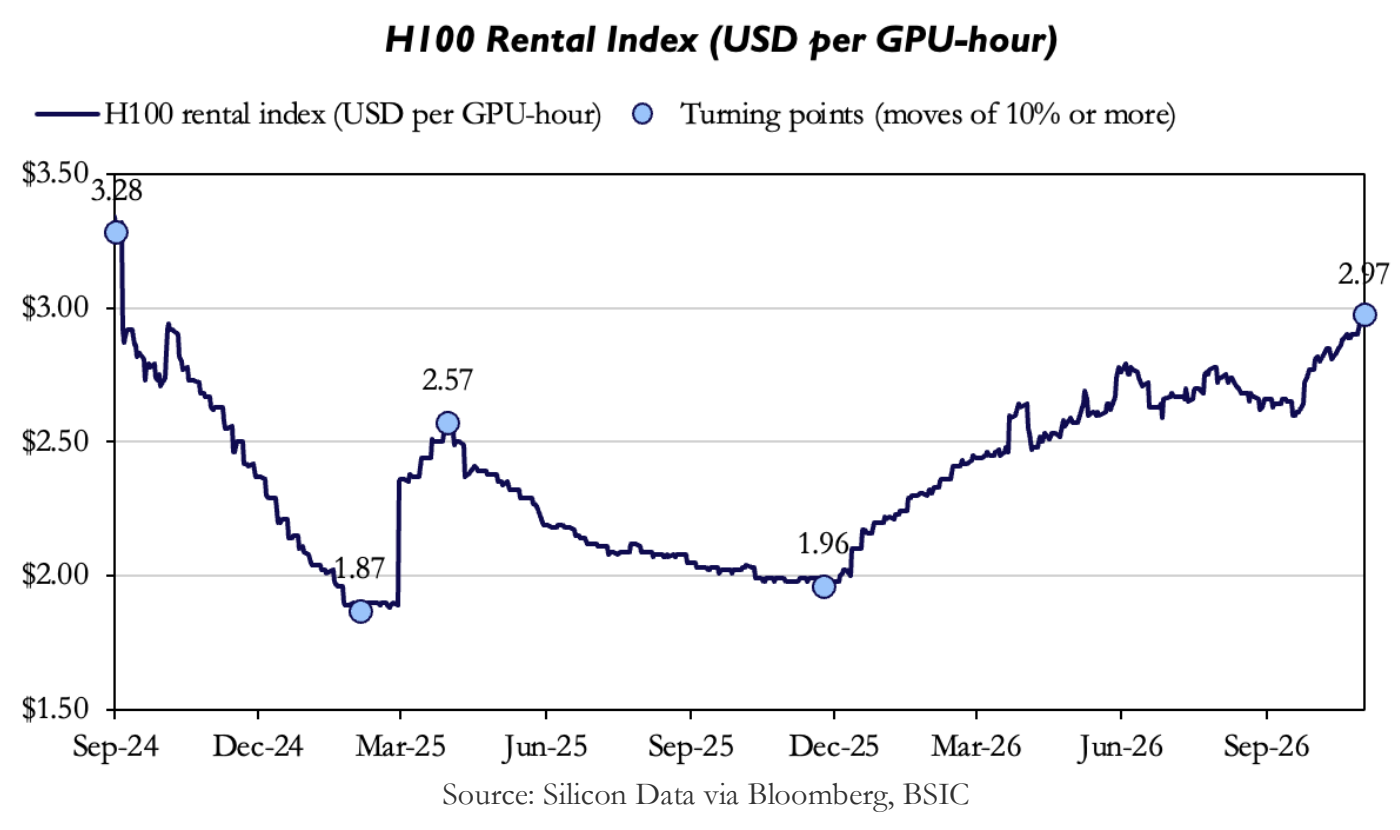
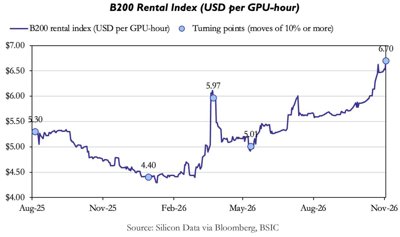
Figure 1 shows substantial declines and recoveries in GPU rental prices. The H100 index fell 43% between September 2024 and February 2025, to $1.87 per GPU-hour. After a brief rebound and a second decline, it rose 52% from late November 2025 to $2.97 in early November 2026. The B200 index has a much shorter history but also increased during 2026, rising from $4.40 in early January to $6.70 in early November.

We forecast next month’s average rental index using observations dated before that month begins. The monthly horizon reflects the averaging basis of CME’s planned compute futures and reduces the influence of day-to-day price movements. We calculate the target as the mean of the daily observations available in each complete calendar month.

Three limitations shape the analysis. First, the histories are short: our sample contains only 25 complete monthly averages for the H100 and 14 for the B200, with fewer observations available for model estimation and evaluation. Second, the historical data have been revised. Silicon Data changed its methodology in December 2025, and our source workbook records a restatement of the H100 history [9]. Although we use observations dated before each forecast month, we cannot fully reconstruct the values available at the time. The backtest therefore uses the currently available historical series. Third, benchmarks differ in geography, hardware configuration, rental terms and data sources. Compute Desk, for example, measures US one-year reserved rental prices [10], so its price levels should not be treated as directly equivalent to an on-demand benchmark.

Which indicators might help?

To organise the forecasting tests, we group candidate indicators into four economic channels: expectations of AI spending, conditions in the rental market, actual compute demand, and the costs of operating and financing the hardware. Table 1 distinguishes the indicators we tested from proposed tests for which we could not obtain suitable historical data.

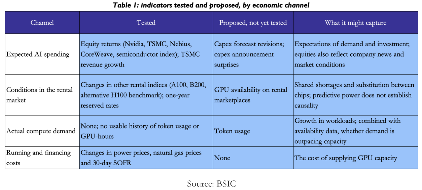
Indicator coverage varies by sample. CoreWeave’s shares, the B200 indices and the one-year reserved rates have shorter histories, so they enter only the B200 test and the weekly H100 check. Most tested indicators are market prices, reflecting expectations or rental-market conditions. Weak results for these proxies do not rule out useful forecasting information in more direct measures of workloads and available capacity, which remain the main gaps in our data.

How we test whether an indicator adds value

We model changes, not levels. Two series that drift over time can look closely related in levels without one being of any use in forecasting the other [11], so every variable enters as a log change, which approximately equals the percentage change when multiplied by 100, for small movements. Let Am+1 be the average rental index in month m+1 and Pm the last index value observed in month m. The quantity we forecast is the change from the month-end index to the following month’s average:

ym+1=lnAm+1-lnPm

For an indicator with value Xm at the end of month m, the predictor is its change over that month:

xm=lnXm-lnXm-1

We then estimate, by ordinary least squares and for one indicator at a time, the regression

ym+1=+xm+m+1

where measures how this month’s move in the indicator is associated with next month’s rental-price change, and m+1 is the part the indicator does not explain. We also estimate one combined model, an economically motivated combination of one indicator from each channel for which we have data: the semiconductor index, the A100 rental index and the power price. For comparison, we estimate two models that use no outside indicator: an intercept-only model, which forecasts the average past change, and one that uses the rental index’s own change in the previous month. The intercept-only model allows us to assess whether an indicator improves forecasting performance beyond simply extrapolating the average historical change.

To approximate forecasting in real time, we restrict predictors to observations dated before the forecast month, subject to the historical-data revisions discussed above. Each predictor xm therefore uses only values dated on or before the last day of month m. Market prices enter on the day they are quoted. Series released with a delay enter on their publication date: TSMC’s monthly revenue, the one such series in our tests, is assumed to be published on the 10th of the following month. Timing does not resolve revisions, however. We use each series as it stands today, including the revised H100 history described in Section 3.1, so the exercise is a backtest on current data and not a reconstruction of what a forecaster saw in real time.

We train on the past and test on the future, re-estimating as time passes [12]. To forecast month m+1, we estimate and on all earlier months, giving am and bm, and then produce a single forecast of next month’s average:

Am+1|m=Pmexpam+bmxm

Because the model is estimated in logs, converting its fitted value back into dollars gives a forecast of the median of next month’s average, not its mean, if errors in logs are symmetric. We back-transform forecasts without a mean adjustment and evaluate their accuracy on the original price scale. The following month, the model is re-estimated using an expanded historical sample. Estimation windows end before the forecast month, although the historical values incorporate retrospective revisions. For the H100 this yields 12 forecasts, from November 2025 to October 2026, each based on 10 to 23 months of training data, depending on the indicator and the forecast date. For the B200 it yields 7, from April to October 2026, each based on 5 to 13 months. The combined model, which has four coefficients, is estimated only where at least 10 months of training data are available, and therefore for the H100 alone. Within each index, all models are scored on the same months. We exclude March 2025 from the main H100 training sample because its unusually large jump may reflect a discontinuity in the revised historical series. We report results including that month as a sensitivity check..

A forecast error is only informative relative to what could be achieved with no model at all. Our benchmark is the last observed price carried forward [13]:

Am+1|m0=Pm

For each model we compute the percentage error of every forecast and summarise it with the root mean squared percentage error:

em+1=Am+1|mAm+1-1

RMSPE=1001N∑em+12

A model outperforms the benchmark over the test period if its RMSPE is lower. We report the difference as a percentage improvement, which is positive when the model does better than the benchmark:

Improvement=1001-RMSPEmodelRMSPEbenchmark

A lower error shows that a model outperformed the benchmark over the test period. With 12 forecasts for the H100 and 7 for the B200, it does not establish dependable predictive value, and the B200 regressions rest on so few months that we treat its results as indicative only. Testing many indicators also makes it likely that one will look useful by chance, so we label the best-performing single indicator as exploratory. For the H100, we check sensitivity to three choices: including March 2025 in the training data, lengthening the test window to 15 months, and lagging the indicators by one further month. Finally, as a supplementary test at a different horizon, we forecast the H100 index one week ahead over the last 52 weeks, or fewer for indicators with shorter histories, measuring errors on weekly log changes against a benchmark of no change.

Results: does additional information improve the forecast?

In the main monthly H100 test, no indicator improved on the benchmark. The figure shows the forecast error of the last-price benchmark, the best indicator in each channel of Table 1, the model with no indicator, the combined model and the weakest of the 15 models tested. Because the best single indicator is identified only after seeing its performance on the test period, we label it exploratory.

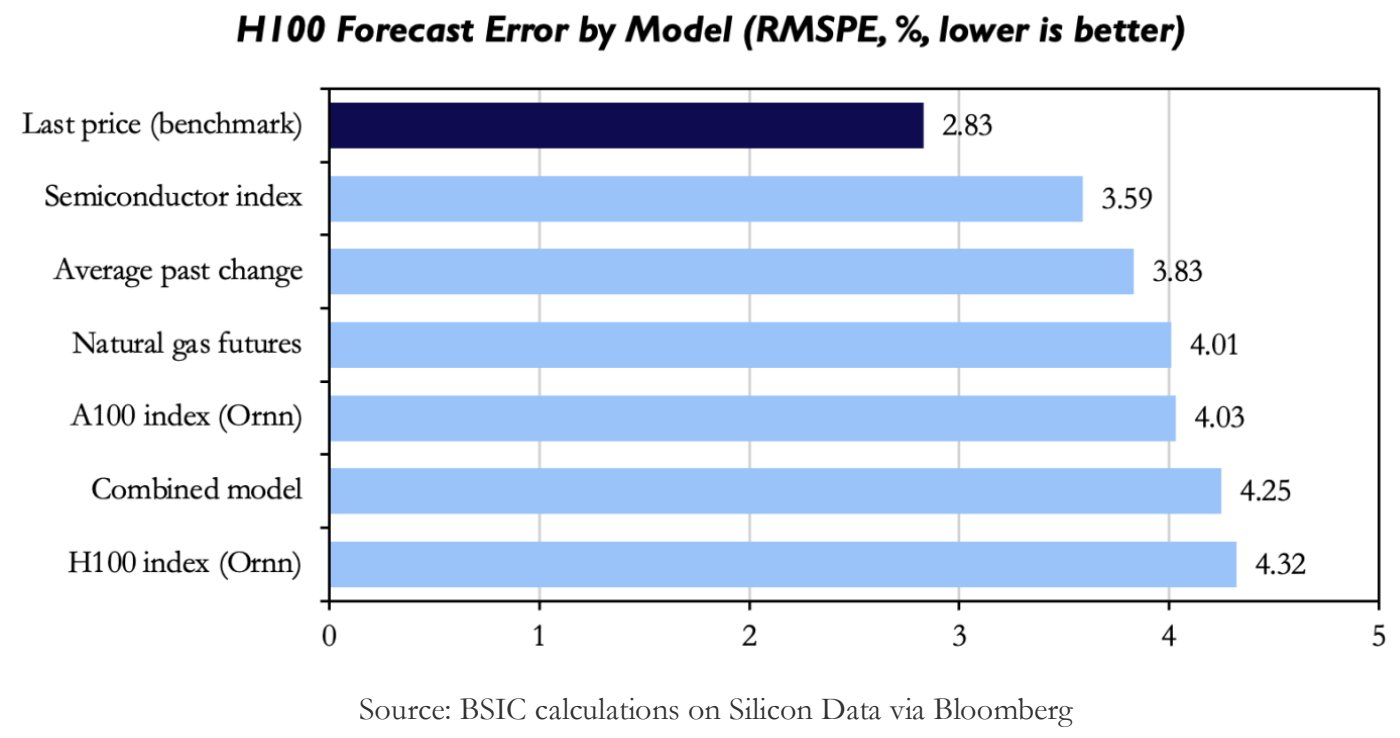
Over the 12 H100 forecasts, carrying the last price forward gave an RMSPE of 2.83%. None of the 15 models did better. The best of them, the semiconductor index, had an error of 3.59%, which is 27% higher than the benchmark’s, and the others ranged up to 4.32%. The combined model, at 4.25%, was worse than two of the three indicators it combines.

Most of this gap does not come from the indicators. The model with no indicator, which forecasts only the average past change, already has an error of 3.83%. H100 rents fell for most of the training period and rose through the test period, so the estimated average change was negative in every forecast, between −2.6% and −0.7% a month, while the actual change over the test months averaged +1.4%. Every model therefore forecast too low, by 2.5% to 3.3% on average, against 1.4% for the benchmark. Measured against the no-indicator model, the semiconductor index lowers the error from 3.83% to 3.59%, and it was closer to the outcome than the benchmark in 5 of the 12 months. A difference of that size is too small to interpret with 12 forecasts.

Was any improvement large enough to matter? For the H100 there was none. For the B200, two of 20 models finished ahead of the benchmark over 7 forecasts. The alternative H100 benchmark published by Ornn gave an RMSPE of 3.13% against 3.66%, an improvement of 15%, and Ornn’s A100 index gave an improvement of 12%. TSMC revenue matched the benchmark and the remaining 17 models were worse. At a representative B200 price of $5.50, these percentage errors correspond to approximately $0.17 and $0.20 per GPU-hour, respectively.

Did the results survive reasonable changes? For the H100, the benchmark stays ahead of every model in all three checks. With March 2025 included in the training data the gap narrows sharply, and the best model reaches 2.91% against 2.83%. This fits the explanation above, since the jump in that month raises the estimated average change. With a 15-month test window, the benchmark’s error is 2.65% and the best model’s is 3.27%. With the indicators lagged by a further month, the best model’s error is 3.60%. The best model is also a different one in each check, TSMC revenue in the first, the semiconductor index in the second and Nebius shares in the third, which is what we would expect if none of them carried a stable signal. The short B200 history limits the robustness checks we can perform and the confidence we can place in them.

Was the uncertainty small enough to distinguish the B200 improvement from chance? The small evaluation sample and the number of models considered prevent us from treating the B200 improvement as established. Testing 20 models on only 7 forecasts makes it more likely that some finish ahead by chance, and each B200 regression is fitted on 5 to 13 months of data. The result also lacks a consistent reading: Ornn’s H100 index helped, but Ornn’s own B200 index and the Silicon Data H100 index both did worse than the benchmark, with errors of 7.35% and 4.75%. We therefore treat the two Ornn indices as preliminary findings requiring validation on a longer sample.

The one-week-ahead test for the H100 gives the same picture. Two of 16 indicators lowered the error of the no-change benchmark, the B200 index by 4% and the one-year reserved B200 rate by 3%, both over fewer than 40 weeks. Two others, the one-year reserved H200 and H100 rates, were within 0.2% of the benchmark, and the remaining 12 were worse.

A separate question is whether rental prices move together within the same month, which is not a forecasting test. Excluding March 2025, the correlation between monthly changes in the H100 index and in the B200 index is 0.54 over 14 months. It is 0.27 with Ornn’s H100 benchmark over 24 months, 0.15 with the A100 index over 24 months and 0.09 with the one-year reserved H100 rate over 13 months. The correlations suggest some shared movement in rental prices, most visibly between the H100 and the B200, but they do not by themselves show that one index predicts another. The weak link between two benchmarks for the same chip is also a reminder that these results describe the Silicon Data index and may not carry over to other providers’ prices.

What these results imply for the curve

The question of this section was whether any available indicator helps to forecast the price on which the futures settle. On the evidence we have, none has established a stable improvement over the last observed price. For the H100, the benchmark was ahead of all 15 models in the main test and in each of the three sensitivity checks. For the B200, two models finished ahead, but over 7 forecasts and without a consistent pattern across related indices.

A few signals remain worth testing again. The two Ornn indices delivered the largest observed reductions in forecast error for the B200, and the B200 index and the one-year reserved B200 rate lowered the error by small margins in the one-week-ahead test for the H100. The semiconductor index improved on the intercept-only model, but its aggregate RMSPE remained above that of the last-price benchmark. We regard all of these as candidates for a later test on a longer sample, not as established predictive relationships.

Several limitations prevent a stronger conclusion. The histories are short, giving 12 monthly forecasts for the H100 and 7 for the B200. The historical series incorporates retrospective revisions, limiting our ability to reconstruct forecasts using the information originally available. For the H100, the early training data were also dominated by falling rents, while prices generally rose during the evaluation period, and this change in direction may help explain the models’ tendency to forecast too low, even as the training sample expanded. Finally, most of the indicators we could test are financial-market prices, which reflect expectations about many things besides the balance between GPU demand and available capacity.

Adding more direct measures of investment, capacity and usage would not resolve the short rental-price history, but it could reduce our reliance on financial-market prices. The most promising additions are the proposed indicators in Table 1. Revisions to analysts’ capex forecasts for the large cloud providers could provide a more direct measure of expected investment than share prices, particularly where AI-related spending can be identified separately. These revisions differ from both capex levels and announcement surprises. GPU availability on rental marketplaces would show how much capacity is available at a given price. Token usage or other workload measures, considered alongside comparable capacity data, could help assess whether demand is growing faster than available supply. We have not yet obtained a usable history for any of them, which is why they remain proposals.

The consequence for pricing is that the available evidence has not established a robust forecasting advantage from the tested indicators, which is a narrower statement than saying that rental prices cannot be forecast. These tests therefore provide no basis for treating any of the estimated relationships as a dependable rule for projecting the settlement index forward [8]. A forecast of the index would not by itself determine a futures price either, since a futures price can differ from the expected settlement value by a risk premium. For that reason, Section 4 compares explicit assumptions about the path of the index and the indicative curves they imply. The last-price benchmark of this section corresponds to the flat scenario, in which the latest observed index value is carried forward. The scenarios show how each assumption changes the curve; they do not turn an uncertain forecast into a single correct futures price.

The Curve Under Scenarios

The previous analysis found that the tested indicators have not established a robust forecasting advantage over the last-observed-price benchmark. These results do not provide a sufficiently strong empirical basis for selecting a longer-term projection model. We therefore project the monthly averages of the H100 settlement index over the next twelve months under four scenarios, each defined by explicit assumptions. These projections illustrate alternative paths, not established fair futures prices. Carrying the latest price forward served as a useful one-month benchmark but extending it across twelve months is a separate assumption.

Table 2 sets out the four assumptions, and the chart that follows shows the expected settlement value that each implies for twelve illustrative monthly settlement periods from November 2026 to October 2027, using the proposed contract specifications. All four start from the index value of $2.97 on 6 November 2026, and each monthly value is the average of the index over the business days of that month. For November 2026 the average combines the values already published with projections for the remaining days.

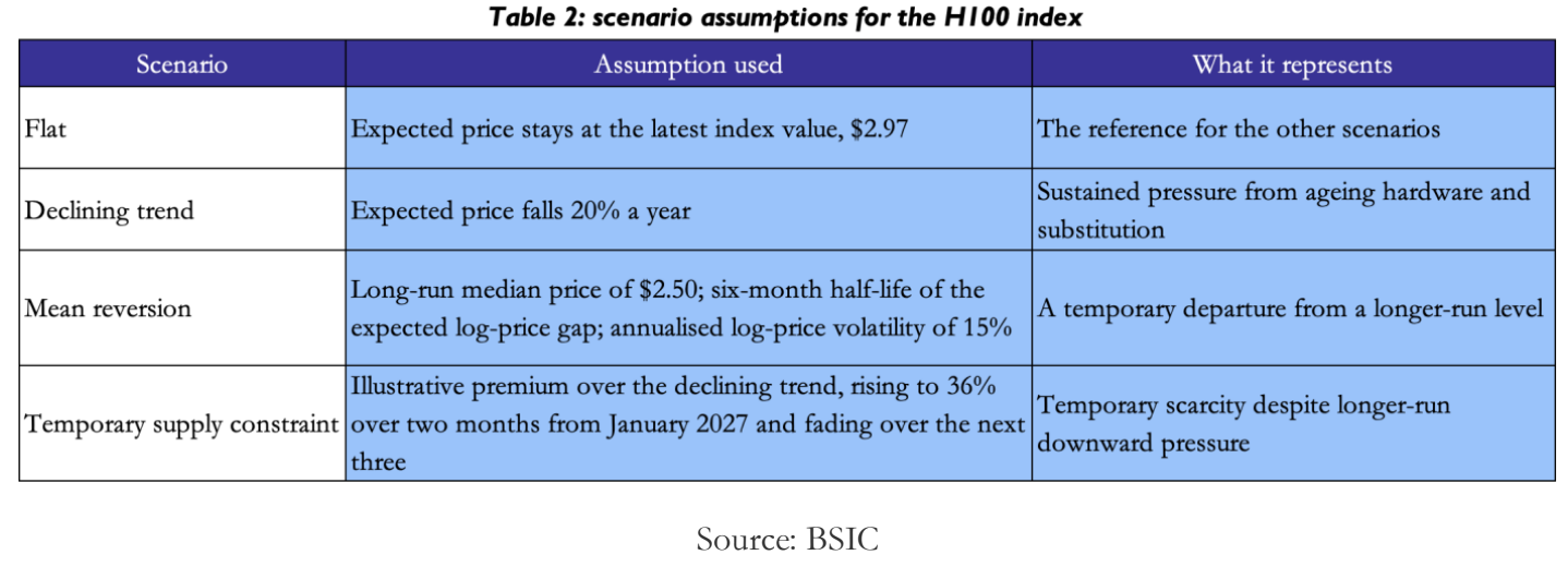
The flat scenario holds the expected price at its latest value and serves as the reference. The declining trend assumes that ageing hardware and substitution by newer chips lower the expected price by 20% a year, an illustrative rate that is moderate beside the 43% fall of the index over 22 weeks in 2024–25. Mean reversion assumes that the log price returns towards a long-run level of $2.50, with half of the gap closing every six months [14]. Both parameters are illustrative assumptions. Estimated half-lives are sensitive to the sample used, and a unit-root test fails to reject the unit-root null, so the historical evidence does not firmly establish mean reversion. The temporary supply constraint is an illustrative period of scarcity added to the declining trend. Its magnitude is informed by the B200 index in early 2026, which rose 36% in about two months and gave back most of the rise within the following two, while its timing and profile are our own assumptions.

None of the four scenarios includes a sustained rise in rents, although the index rose 52% in the year to November 2026. That omission is a choice of ours and not a result of Section 3.

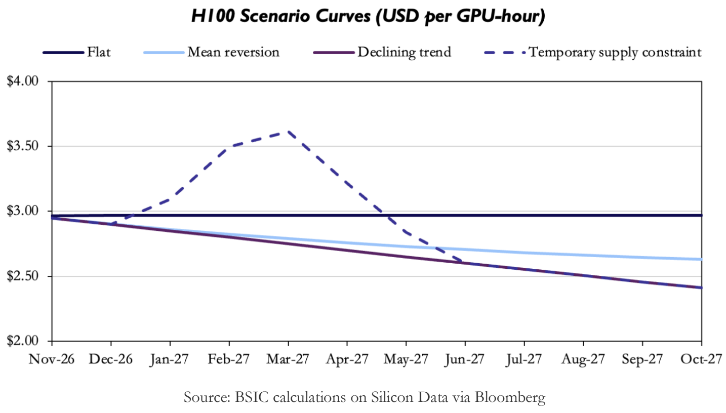
The curves start close together and separate with maturity. For December 2026 the four projections lie within $0.07 of one another, about $50 on one proposed contract of 730 GPU-hours. Leaving the supply constraint aside, the gap widens steadily, to $0.56 between the flat and declining curves for October 2027, about $410 per contract. The supply constraint behaves differently. It lifts the March 2027 value to $3.61, which is $0.86 or 31% above the declining trend, and then fades, so that the two curves virtually coincide by June 2027. A temporary disruption therefore matters most for the months that cover it, while a persistent trend matters most for the most distant ones.

One market reference offers context. The one-year reserved H100 rate quoted by Compute Desk was $2.78 on the same date, close to the average of the mean-reversion curve across the twelve months, $2.76. The proximity does not validate that scenario: a reserved rate reflects commitment terms, access to capacity and the provider’s own benchmark construction, and a one-year reservation does not cover exactly the same twelve months.

These differences measure sensitivity to the assumptions chosen. They are not confidence intervals and they do not show which scenario is most likely. The curves are projections of the settlement index before any risk premium, not fair futures prices.

Conclusion 

The evidence available at the time of writing did not establish a robust forecasting advantage from the tested indicators. Across 12 monthly H100 forecasts, carrying forward the last observed price produced a root mean squared percentage error of 2.83%, outperforming all 15 models, with this result holding across the sensitivity checks. For analysis of B200 rental pricing, two of 20 models outperformed the benchmark; however seven forecasts were insufficient to establish dependable predictive value. 

Interpretation is limited by short histories, revisions to historical data and the shift from falling to rising rents. Furthermore, most tested indicators reflect financial market expectations rather than directly measuring capacity or workloads. These findings support assessing explicit alternative paths for the settlement index, without concluding that compute rental prices cannot be forecast using other methodologies.

The evidence does not rank the four scenarios, but their comparison shows how assumptions shape the projected settlement curve. For October 2027, projections range from $2.41 to $2.97 per GPU-hour, a difference of about $410 per proposed contract of 730 GPU-hours. Under the temporary supply constraint, the March 2027 projection reaches $3.61 before the curve returns to the underlying declining path. Persistent assumptions therefore affect distant maturities, while a temporary disruption concentrates its impact in the affected months. These are projections of the settlement index before any risk premium, not estimates of fair futures prices.

In future parts of this article, scenario parameters will be calibrated, curve uncertainty will be measured, and compute futures’ risk premia will be estimated. Additionally, the gap between the settlement index and what a user pays for capacity will be examined. Further empirical work will incorporate revisions to hyperscalers’ capex forecasts, alongside measures of GPU availability and token usage. The B200 results will be reassessed with a longer sample. 

Once the contracts are approved and traded, listed prices can be compared with the scenario curves, with differences potentially reflecting both market expectations and risk premia. Evidence to refine the framework will hence be provided without identifying a single correct forecast from market prices alone. 

References

1. Yu, Yuhua and Hou, Steve, “Cash-Settled Compute Futures”, 2026. 
2. Marchese, John, “Voluntary Extension of Review Period for New York Mercantile Exchange, Inc. Submission of Two (2) Compute Futures Contracts…”, 2026.
3. Dealroom.co, “Wall Street’s GPU futures slip to 2027 as the CFTC extends its review of CME’s Nvidia rental contracts…”, 2026.
4. CME Group, “CME Group and Silicon Data to Launch Compute Futures on October 5 to Unlock New Way to Hedge AI Risks”, 2026.
5. Intercontinental Exchange, “ICE and Ornn to Launch GPU Compute Futures Contracts”, 2026.
6. Intercontinental Exchange, “ICE and NATIVX to Launch Energy-Normalized Compute Futures Contracts”, 2026.
7. Shen, Muyao, “Jump, DRW Bet on New Compute Market as AI Boom Faces Scrutiny”, 2026.
8. CME Group, “Compute Futures”, 2026
9. Silicon Data, “Silicon Data Announces Major Revision to A100 & H100 Rental Indices, Launches First-Ever B200 Index, and Introduces New Hyperscaler Rental Benchmarks”, 2025
10.  Compute Desk, “Index Methodology”, 2026
11.  Granger, Clive W. J.; Newbold, Paul “Spurious Regressions in Econometrics”, 1974
12.  Welch, Ivo; Goyal, Amit “A Comprehensive Look at the Empirical Performance of Equity Premium Prediction”, 2008[14]Schwartz, Eduardo S. “The Stochastic Behavior of Commodity Prices: Implications for Valuation and Hedging”, 1997
13.  Meese, Richard A.; Rogoff, Kenneth “Empirical Exchange Rate Models of the Seventies: Do They Fit Out of Sample?”, 1983
14.  Schwartz, Eduardo S. “The Stochastic Behavior of Commodity Prices: Implications for Valuation and Hedging”, 1997