Liquidity and the Value of Anticipating Selling Pressure in Optimal Execution: An Almgren–Chriss Study

Download PDF

Introduction

For a fund, deciding to sell is only part of the challenge. In this article, we explore how to execute large equity sales efficiently, balancing market impact against the risk of adverse price movements, and how liquidity and the ability to anticipate selling pressure influence that decision.

When a fund must liquidate a block of shares before a fixed deadline, whether due to investor redemptions, an index deletion, a risk-limit breach or a margin call, the quantity and the horizon are already determined. What remains is how to distribute sales over time. Selling quickly increases market impact, potentially depressing execution prices, while selling slowly reduces immediate trading costs but leaves the unsold position exposed to market risk. Almgren and Chriss [1] formalised this trade-off within a mean–variance framework, deriving optimal liquidation schedules and an efficient frontier of execution strategies. Their static optimal execution model provides the foundation for our analysis.

The challenge becomes more complex when selling pressure extends beyond a single investor. Redemptions may affect funds with similar portfolios simultaneously, index deletions can force multiple trackers to sell the same securities, and deleveraging episodes may push investors towards the exit at the same time. A fund anticipating such pressure faces an additional decision: should it accelerate its sales to avoid a potential price decline, or maintain its original execution schedule? Crucially, this decision must be made using a forecast that may prove inaccurate.

Research Framework and Contribution

We organise the analysis around two hypotheses. H1 (Liquidity and Efficient Frontiers) asks whether more liquid securities, ranked by Amihud [4] illiquidity, exhibit more favourable Almgren–Chriss efficient frontiers than less liquid securities. H2 (The Economic Value of Anticipating Selling Pressure) investigates how a predictable negative price drift affects optimal liquidation, how the value of incorporating it depends on stock liquidity, and how sensitive that value is to forecast errors.

Our analysis draws on two strands of financial research. The first concerns optimal trade execution. Bertsimas and Lo [5] studied how to minimise the expected cost of executing large orders, while Almgren and Chriss [1] incorporated execution risk into the optimisation problem, deriving optimal liquidation schedules and their efficient frontier. Subsequent research extended the framework to nonlinear market impact (Almgren [2]), resilient limit-order books (Obizhaeva and Wang [13]) and conditions preventing price manipulation (Gatheral [10]). Almgren, Thum, Hauptmann and Li [3] estimated market impact using institutional orders, while Lorenz and Almgren [12] examined the optimality of static execution strategies. Cartea, Jaimungal and Penalva [8] provide a comprehensive treatment of the field. The second strand examines price pressure generated when multiple investors trade in the same direction, including index changes (Shleifer [15]; Harris and Gurel [11]), mutual fund fire sales (Coval and Stafford [9]) and strategic trading around distressed liquidations (Brunnermeier and Pedersen [6]; Carlin, Lobo and Viswanathan [7]).

The study lies at the intersection of these two strands of research. Rather than developing a new market impact model, we retain the linear Almgren–Chriss framework and its impact calibration approach, using the price-pressure literature to motivate hypothetical drift scenarios rather than to estimate actual selling pressure. Our contribution is threefold. First, we apply the model to a cross-section of US equities classified by Amihud illiquidity, examining how liquidity shapes efficient execution frontiers. Second, we quantify how the economic value of anticipating selling pressure varies across liquidity groups. Third, we extend the analysis to imperfect drift forecasts, deriving an analytical relationship between forecast accuracy and execution value in the unconstrained regime and examining how non-negative trading constraints modify this relationship.

The remainder of the article introduces the Almgren–Chriss framework and its calibration to CRSP data, before examining the relationship between liquidity and efficient execution frontiers. We then investigate the economic value of anticipating selling pressure, the consequences of forecast errors and the role of trading constraints. Finally, we discuss the implications for execution desks and the limitations of our analysis. All reported execution costs and benefits are model-implied rather than realised trading outcomes.

The Almgren–Chriss Framework

A fund holds X shares and must sell them over a horizon T divided into N periods of length τ = T/N. In our application T is five trading days and τ is one day. The schedule is described by the holdings xk after period k, with x0 = X and xN = 0, or equivalently by the sales nk = xk−1 − xk. Almgren and Chriss model the mid price as an arithmetic random walk,

where σ is the price volatility in dollars per share per square root of a day, ξk are independent standard shocks and g is permanent impact. The price the fund actually receives is lower than the mid price by the temporary impact h(v) of its selling speed v = nk/τ. With linear temporary impact h(v) = ε + ηv, ε is a fixed cost per share (half the bid–ask spread plus fees) and η measures how much the price received falls per unit of selling speed.

The implementation shortfall, the difference between the paper value XS0 and the cash actually received [14], is random. The cash received in period k is nk times the execution price, Sk−1 − h(nk/τ), and the mid price itself has moved by the accumulated shocks since the start. Summing over periods and rearranging, the shortfall equals the impact paid on each sale minus the price changes earned or lost on the shares still held, Σ σ√τ ξk xk. Because the shocks have mean zero and are independent, the expected shortfall contains only the impact terms and the variance only the holdings. With permanent impact set to zero (we explain why below), its mean and variance are

The impact term is convex in each sale, so spreading the sale evenly minimises expected cost; the variance grows with every share still held, so selling early minimises risk. The fund resolves the conflict by minimising E + λV, where λ ≥ 0 measures its aversion to risk. Two extreme strategies bracket every solution. Selling at a constant rate, nk = X/N, is the TWAP strategy of market practice; it has the lowest possible expected cost, εX + ηX²/T, but leaves the position exposed for the whole horizon, with variance ⅓ σ²X²T (1 − 1/N)(1 − 1/(2N)). Selling everything in the first period eliminates the risk but pays εX + ηX²/τ, an impact cost N times larger. The optimal schedules lie between the two. Setting the derivative of E + λV with respect to each holding xk to zero gives, for every interior period,

a linear second-order difference equation: the “acceleration” of the holdings is proportional to the holdings themselves, with a coefficient that measures how much the fund dislikes risk relative to how much fast selling costs. With the boundary conditions x0 = X and xN = 0, its solution is the celebrated hyperbolic-sine schedule

The inverse of κ is what Almgren and Chriss call the half-life of the trade, the intrinsic time scale over which the fund would unwind the position if it had no deadline. Strictly, 1/κ is a characteristic decay time rather than a half-life, since a position decaying exponentially at rate κ halves after (ln 2)/κ; we keep their term. The single number κT, the ratio of the deadline to this time scale, governs the shape of the schedule. When κT is close to zero the fund sells almost evenly, the TWAP schedule that minimises expected cost; when κT is large it sells most of the position at the start. Since κ² is approximately λσ²/η, a stock whose temporary impact is high relative to its volatility is sold more evenly: in Almgren and Chriss’s words, a trader will execute a more liquid basket more rapidly than a less liquid one. Tracing the optimal schedule for every λ produces the efficient frontier, the lowest expected cost attainable for each level of variance. Every schedule fixed in advance lies on or above it. The frontier is smooth and convex, and at its TWAP end it is flat: a first-order reduction in variance costs only a second-order increase in expected cost. Unless the fund is exactly risk neutral, it therefore always pays to sell somewhat faster than TWAP, which is why Almgren and Chriss argue that a strictly risk-neutral schedule never makes sense. They also note that the curvature of the frontier near its minimum is itself a measure of the liquidity of the security, an idea that H1 develops by comparing whole frontiers across stocks.

Two further properties of the model matter for this article. First, the schedule is time-homogeneous: if the fund re-solves the remaining problem after any number of days, with the same objective and unchanged parameters, it recovers the continuation of the original plan. With independent price increments and known parameters, the fund learns nothing during the sale that would change its plan, so a static schedule chosen at the start is optimal in the mean–variance sense the model uses. Second, the schedule does not depend on the position size X, since both the impact cost and the variance scale with X². The schedule changes only if the fund has information about the future that the base model excludes. A predictable drift in the price is the simplest such information, and Almgren and Chriss themselves show how to use it. We return to it after testing H1.

Data and Calibration

Data and universe. We use the CRSP daily stock file in its CIZ format [16]. The universe is formed on 2 January 2025, the first trading day of the year, using only information available on that day: the 3,000 largest US common shares listed on the NYSE, Nasdaq and NYSE American, by market value, trading at a price of at least $5. The universe is formed without conditioning on later survival, which mitigates survivorship bias, although the minimum-data requirement below may exclude securities that disappear or trade too rarely during the estimation period. Every parameter is then estimated on the following trading days up to 30 June 2025, and a stock must have at least 100 usable days out of about 120 to enter the study, leaving 2,814 stocks.

Cleaning and corporate actions. We use closing bid and ask quotes, discarding quotes that are missing, locked or crossed, or wider than 20% of the midpoint. Days without a trade are excluded from the Amihud measure. Because the calibration is expressed per share, we adjust prices, quotes and volumes for splits, rebuilding CRSP’s cumulative adjustment factors from its daily price factor and checking them against its price return excluding dividends; total returns are used as reported.

Liquidity measures. For each stock we estimate four quantities on the training period: the median relative closing spread s0 = (Ask − Bid)/Mid, using the median so that a few days with very wide quotes do not dominate; the volatility of daily returns σr; the average daily share volume ADVsh; and the Amihud ratio

the average absolute return per $1m traded. Amihud measures how far the price moves for each dollar that changes hands, a price-response dimension of liquidity related to, but distinct from, the spread. Amihud plays only one role: it ranks stocks into four quartiles, from Q1 (most liquid) to Q4 (least liquid). It does not enter any execution cost, which depends on the spread, the volatility and the volume through the calibration below.

Calibration. We follow Almgren and Chriss’s rule of thumb: the fixed cost equals half the spread, and “for each one percent of the daily volume we trade, we incur a price impact equal to the bid-ask spread”. With Spreadabs = s0 S0 the absolute spread,

Share volume, not dollar volume, is the correct denominator: η multiplies a speed in shares per day and must return a price in dollars per share. The order is X = 10% of ADVsh, sold over five days, or 2% of daily volume per day at TWAP. Permanent impact is set to zero: with linear permanent impact its contribution is identical for every schedule, so it does not affect which schedule is optimal, and it cannot be separated from temporary impact without the fund’s own orders.

Normalisation. To compare stocks of very different size and price, costs are measured per dollar of position value X S0 and expressed in basis points. Writing wk = nk/X for the fraction sold on day k and hk for the fraction still held, the normalised expected cost and variance are

The volume cancels because the order is a fixed fraction of it, and the price cancels from every term. The risk aversion becomes a pure number, λrel = λ X S0. We choose it once, on training data, so that the median stock has κT = 1, an intermediate urgency at which the half-life of the trade equals the deadline:

With a common λrel each stock’s urgency becomes an output, κ²∝ σr²/s0: volatile stocks with tight spreads are sold quickly, calm stocks with wide spreads slowly. It is a modelling convention, not an estimated preference, and H1 does not depend on it.

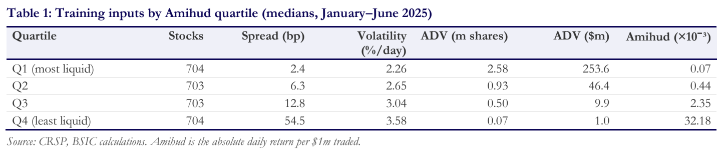
Table 1 describes the four quartiles. The ranking by Amihud lines up with every other dimension of liquidity: the median spread rises from 2.4bp in Q1 to 54.5bp in Q4, average dollar volume falls from 254m to under 1m per day, and volatility rises from 2.3% to 3.6% per day. Less liquid stocks are therefore both more expensive to trade and riskier to hold, which is what makes their frontiers interesting.

Do Liquid Stocks Have Better Frontiers?

Building comparable frontiers. H1 asks whether securities classified as more liquid by Amihud have lower minimum expected execution costs at comparable levels of liquidation risk. Although a common risk-aversion parameter allows us to compare optimal liquidation decisions across stocks, it generally produces different levels of execution risk. Since our objective is to assess how liquidity affects the cost of achieving a given risk level, we instead compare efficient frontiers at common levels of normalised risk. We therefore build each stock’s frontier directly, by minimising expected cost subject to a maximum level of normalised risk r*:

The problem is convex, and its Karush–Kuhn–Tucker conditions are those of Almgren and Chriss’s problem with the multiplier of the risk constraint playing the role of λ. The solution is therefore the sinh schedule at the value of κ that makes the risk constraint bind, which we find by bisection. Each frontier runs from selling everything on day one (zero risk, cost 10.5 s0) to TWAP (cost 2.5 s0, risk σr√1.2).

The normalisation reveals a simple structure. Dividing by the spread and measuring risk in units of volatility,

where φ is the same decreasing function for every stock. The spread scales a frontier vertically, and volatility stretches it horizontally: at a given risk limit a more volatile stock must sell faster and therefore pays more. A lower frontier thus requires a narrower spread, a lower volatility, or a favourable combination of the two. Amihud illiquidity does not enter the formula, so H1 is an empirical question about how spreads and volatilities line up with the Amihud ranking, not an identity.

Common risk levels. Stocks differ in volatility, so their attainable risk ranges differ, and frontiers can be compared only where they overlap. We use 41 equally spaced risk levels from 0 to 162.7bp, the smallest across quartiles of the 10th percentile of TWAP risk. The calmest stocks, whose TWAP risk falls below this level, are excluded so that every risk level compares the same 2,681 stocks, each on its own frontier and without extrapolation. The quartile frontier at each risk level is the median of its stocks’ minimum costs. The common range has a price: it covers about two thirds of the median TWAP risk in Q1 (248bp) but only about 40% of it in Q4 (392bp), so the comparison concentrates on the urgent part of the frontiers, where the fund sells faster than TWAP. That is also the part of the frontier where Almgren and Chriss’s argument says a risk-averse fund should be.

A worked example shows how the two ingredients interact. Consider a stock A with a 5bp spread and 1.5% daily volatility and a stock B with a 20bp spread and 3% volatility, and a common risk limit of 100bp. A meets the limit by selling 43.8% of the position on day one and tapering off, at an expected cost of 17.0bp. B is twice as volatile, so it must sell 68.4% on day one to stay within the same limit, and its expected cost is 113.9bp. Of that cost, 68.0bp, four times A’s, simply reflects its four times wider spread; the remaining 45.9bp arises because B’s higher volatility forces it to sell faster.

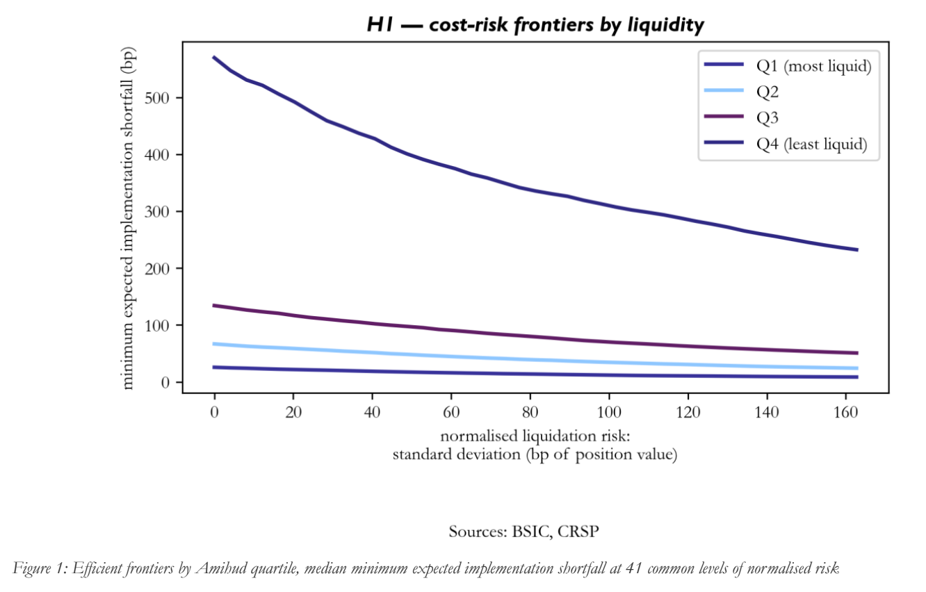
Figure 1 shows that the efficient frontiers are consistently ordered by liquidity. At every common risk level, less liquid stocks face higher expected execution costs, with no crossings between quartiles. Table 2 quantifies these differences. At zero risk, median execution costs range from 25.7bp in Q1 to 569.9bp in Q4, a 22-fold difference. At the highest common risk level, the gap increases to 27 times, as liquid stocks can reduce execution costs more effectively when allowed to take additional risk.

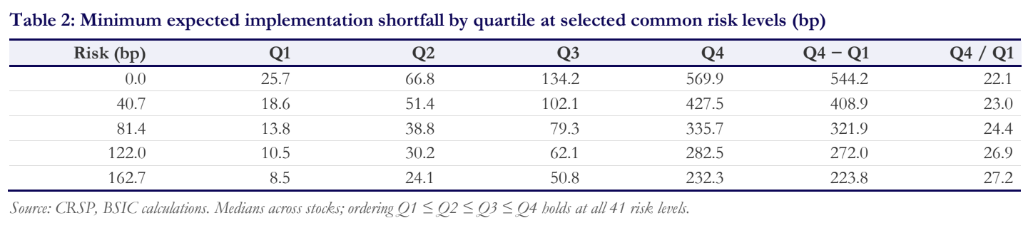
Spread or volatility? The scaling relation lets us split the gap between quartiles into its two sources. At zero risk the shape factor φ equals 10.5 for every stock, so the whole gap reflects spreads. As the risk limit is relaxed, φ starts to differ across quartiles because less liquid stocks are also more volatile. Table 3 reports the median φ by quartile: at the largest common risk level it is 3.33 in Q1 and 4.74 in Q4. Volatility therefore makes Q4 about 1.4 times more expensive than Q1 for a given spread, while the spread itself is 23 times wider. The spread is by far the dominant source of the gap, and volatility is the reason the ratio of the frontiers rises from 22 to 27 as risk increases.

Having established how liquidity shapes model-implied execution costs, we now turn to the value of anticipating selling pressure.

Anticipating Selling Pressure: Almgren–Chriss with a Drift

Selling pressure as a hypothetical drift. When many investors sell the same stock at the same time, their combined selling may depress the price while it lasts, as documented around mutual fund fire sales [9] and index changes [11]. A fund that anticipates such pressure may expect the price to fall during its own liquidation. We do not claim that other investors’ selling necessarily produces a negative drift, nor one of a given size. We treat the drift as an exogenous, hypothetical scenario that the fund takes as given, while its own impact remains the temporary impact calibrated above:

The normalised drift α is expressed in bp of the price per day. Daily CRSP data reveal no other investor’s orders, so α is not estimated: it takes the values 0, −2, −5, −10, −20 and −50bp per day, with −10bp per day (about −50bp over the five trading days) as the reference scenario. The grid spans pressure from a fraction of a typical spread to that of a crowded exit.

The optimal schedule. On each day the fraction still held, hk = 1 − Σj≤k wj, gains ατ in expectation, so the drift adds a term linear in the holdings to the expected cost while leaving the variance unchanged:

The drift term follows directly from the shortfall decomposition above: each share still held at the end of period k earns the expected price change ατ Σ xk, which per dollar of position is ατ Σ hk. With α < 0 the term is a cost that grows with every share the fund keeps. Almgren and Chriss solve the unconstrained version. The first-order condition becomes the difference equation of the previous section with the holdings measured relative to x̄ = α/(2λσ²), the holding a mean–variance investor would choose in a static portfolio problem, and the optimal trajectory is

the zero-drift sinh schedule plus a correction proportional to x̄. The bracket is zero at both ends of the horizon and positive in between, and the correction does not depend on the size of the position. With α < 0, x̄ is negative and the fund sells faster. Here x̄ is a reference level in the formula, not a holding, so a negative x̄ does not by itself make the schedule infeasible: what a liquidation requires is that every sale is non-negative, nₖ = xₖ₋₁ − xₖ ≥ 0. For a sufficiently strong negative drift the unconstrained formula implies negative sales on the last days, that is, buying back shares, which a liquidation cannot do. We therefore impose the non-negative sales constraint wk ≥ 0 and solve the convex quadratic programme exactly, enumerating the possible sets of days with zero sales. The solution coincides with Almgren and Chriss’s formula whenever that formula gives non-negative sales. The schedule is still chosen at the start, so the strategy remains static in their sense: the drift changes the plan, not the need to re-plan.

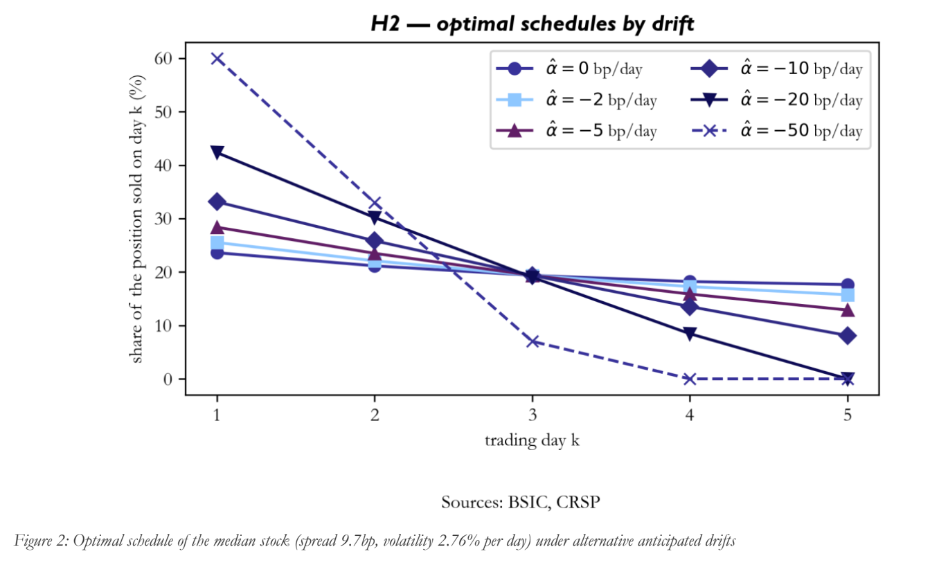
Figure 2 shows the effect on the median stock. Without a drift it sells 23.6% of the position on day one and 17.6% on day five. At −10bp per day the first sale rises to 33.1% and the last falls to 8.1%; at −20bp the fund sells nothing on the last day; at −50bp it completes the sale in three days, selling 60.0%, 33.0% and 7.0%. The non-negative sales constraint is therefore not a technicality: it is what turns a strong view into an early completion of the sale.

The gain due to drift. Almgren and Chriss measure the value of a correct view as the improvement in the objective from following it. Let w*(α) denote the optimal schedule for drift α. Comparing the zero-drift schedule (strategy A) with the drift-informed schedule (strategy B), both evaluated under the true drift α,

G is non-negative by construction, since w*(α) minimises Uα over a set that contains w*(0). Almgren and Chriss bound it from above by the expected price change the adjusted holdings capture,

and since the adjustment h*(α) − h*(0) is itself proportional to α, the bound is quadratic in α. Our own algebra adds that, when the constraint does not bind, the gain is exactly half of their bound, which gives a closed form:

The gain grows with the square of the drift, falls with risk aversion and volatility, which make the fund sell quickly anyway, and rises with urgency κT, which is high when the spread is small relative to volatility. Since Amihud quartiles differ in both spread and volatility, the formula alone does not say which quartile gains more. Almgren and Chriss found the gain negligible for plausible positive drifts; the quadratic dependence means that their conclusion need not carry over to the larger price pressure that crowded selling can create. The closed form holds only in the unconstrained regime. G itself is defined as the difference in the objective, and whenever the constraint binds we compute it from the constrained optimal schedules; every value of G reported below is computed in this way.

What Is It Worth to See the Selling Coming?

Table 4 reports the main analysis across all stocks. At the reference drift of −10bp per day (about −50bp over the five trading days), the median stock raises its day-one sale from 24.4% to 34.6% of the position, and anticipating the drift lowers the objective by 2.2bp, or 4.8% of the objective of the zero-drift schedule. The quadratic shape is clearly visible: halving the drift to −5bp cuts the gain to 0.56bp, while −20bp raises it to 8.8bp and −50bp to 41.6bp, more than a third of the objective. For mild pressure Almgren and Chriss’s conclusion holds: a gain of 0.1bp at −2bp per day is economically irrelevant next to a median zero-drift expected cost of about 25bp. For strong pressure it does not.

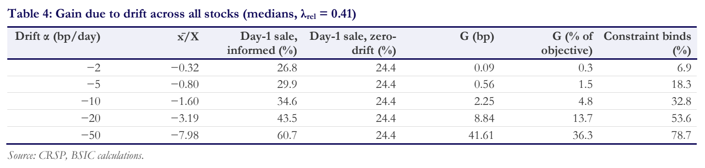
The last column shows how quickly the non-negative sales constraint becomes the rule rather than the exception: it binds for a third of the stocks at −10bp per day and for almost four in five at −50bp. The value of x̄/X also shows that x̄ alone does not decide whether the constraint binds. At the reference drift the median x̄/X is −1.6, yet the unconstrained schedule remains feasible for two thirds of the stocks, and in Q4, where the median x̄/X is −0.95, it remains feasible for every stock. Whether a sale turns negative depends on x̄ together with the urgency κT, which is why the constraint binds mostly in the liquid quartiles.

The role of liquidity. Figure 3 and Table 5 split the gain by Amihud quartile, and the result is the reverse of H1. The most liquid stocks gain most from anticipating selling pressure: at the reference drift the median gain is 6.2bp in Q1, 3.4bp in Q2, 1.8bp in Q3 and 0.4bp in Q4, a fourteen-fold difference. The ordering holds at every drift on the grid. The mechanism is urgency. The median κT falls from 1.59 in Q1 to 0.45 in Q4: a stock with a 2bp spread can move its sales forward cheaply to escape a falling price, whereas a stock with a 55bp spread pays dearly for every share it brings forward and so stays close to TWAP whatever it expects. The gap narrows for very strong drifts, from fourteen-fold at −10bp to about five-fold at −50bp, because the constraint caps the response of liquid stocks first.

 

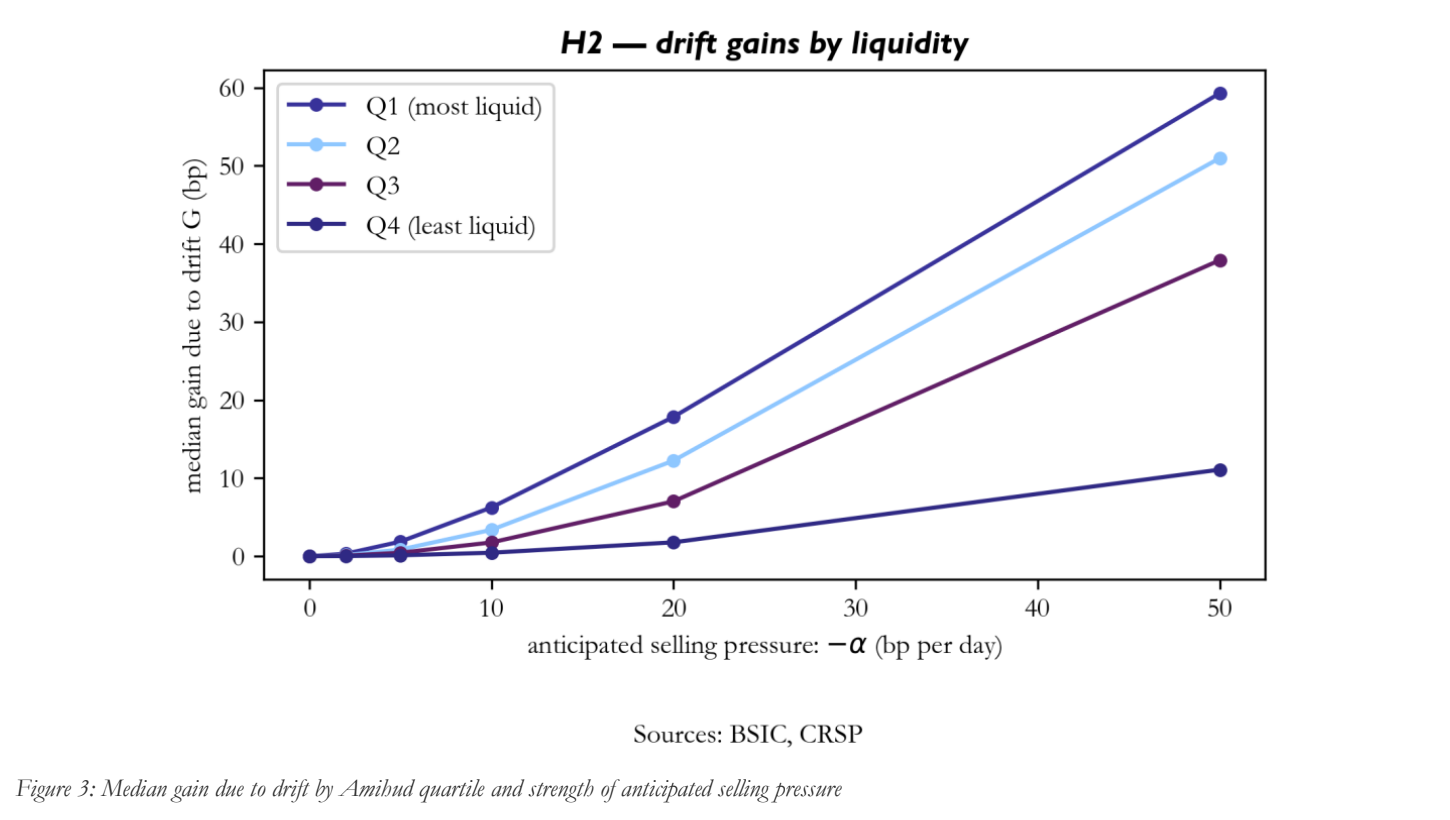
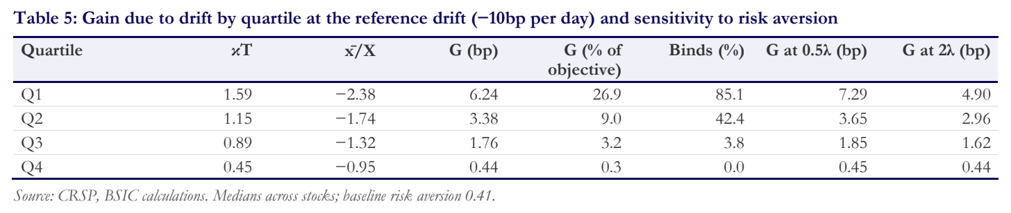
Relative to the cost of the sale the contrast is even sharper. For a Q1 stock, anticipating a −10bp drift is worth about a quarter of the objective; for a Q4 stock it is worth 0.3%. Combined with H1, this gives a simple picture: liquid stocks are cheap to sell, and information about the price matters a great deal for them; illiquid stocks are expensive to sell, and the same information barely changes what they should do.

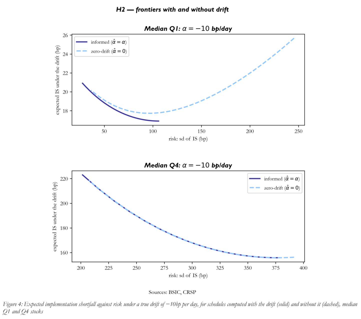
Better frontier or better point? Figure 4 traces, for the median Q1 and Q4 stocks, the frontier of the drift-informed schedules and that of the zero-drift schedules, both evaluated under the reference drift. For the Q1 stock the two frontiers separate: under a falling price, the slow zero-drift schedules become dominated, since waiting is both risky and expensive, and over the range of risk the two share, the informed frontier lies below the zero-drift one. For the Q4 stock the two curves are indistinguishable. Ignoring selling pressure thus puts a liquid stock on a worse frontier, whereas for an illiquid stock it costs almost nothing, because selling faster is too expensive to be worth it.

Risk aversion. Halving the risk aversion raises the gain in Q1 from 6.2bp to 7.3bp and doubling it lowers the gain to 4.9bp; in Q4 the gain barely moves. A less risk-averse fund reacts more strongly to the same drift, but a more risk-averse one already sells quickly and leaves less of the position exposed. The ranking across quartiles is the same at all three levels, so the liquidity result does not depend on the chosen λrel.

When the Forecast Is Wrong

Everything so far assumes that the fund knows the drift. A real forecast of selling pressure can be wrong in size or in sign, and a schedule built on a wrong forecast is not guaranteed to beat one that ignores the drift. This section extends Almgren and Chriss’s analysis to that case.

Forecast and true drift. We separate the drift the fund forecasts, ˆ, which it uses to choose its schedule w*, from the drift that governs the price, true, under which the schedule is evaluated. The schedule is chosen once and never re-optimised with true, which the fund does not know when it plans. Two measures follow. The loss relative to perfect information,

compares the forecast schedule with the one the fund would have chosen had it known the truth. The benefit of following the forecast,

compares it with the schedule that ignores selling pressure altogether. B answers the practical question, whether the fund is better off acting on its forecast than ignoring it, and unlike G and L it can take either sign. Adding and subtracting Utrue(w*(true)) gives the decomposition B = L(0, true) − L(ˆ, true): the benefit of a forecast is the loss from ignoring the drift minus the loss that remains after acting on the forecast. A perfect forecast has L = 0 and B = G, a forecast of zero has B = 0, and when there is no drift any non-zero forecast has B = −L(ˆ, 0) < 0. Equivalently, B = G − L, where G is the gain from a perfect forecast, so B ≤ G: no forecast is worth more than a perfect one. These identities rest only on definitions and optimality, so they hold whether or not the constraint binds.

Two sign results that hold even when the constraint binds. The closed-form rule below requires the constraint to be slack, but two weaker results do not. Write the objective as Uaw=Cw-a Hw, where C collects the impact costs and the risk penalty and Hw=khk is the position’s exposure to the drift; the feasible set, kwk=1 and wk0, is the same for every forecast. Let w0=w*0 and wf=w*, with ΔC=Cwf-Cw0 and ΔH=Hwf-Hw0. Because w0 minimises C, ΔC0; because wf minimises U, ΔC ΔH. Since B=-ΔC+true ΔH, writing =r true gives

If 0<r1, the second inequality gives true ΔH0 and the first gives B0; a zero forecast gives B=0. If r<0, then true ΔH0 and B=-ΔC+true ΔH0. A forecast with the right sign that does not overstate the drift can therefore never do worse than ignoring it, and a forecast with the wrong sign can never do better, whether or not the constraint binds. These are simple consequences of optimality over a common feasible set with a drift that enters the objective linearly, not new results, and they say nothing about forecasts that overstate the drift (r>1). In our sample all 50,652 stock–pairs with 0<r1 have B>0, including 22,205 in which the constraint binds, and all 56,280 pairs with r<0 have B<0.

A closed-form rule. When the constraint does not bind, the problem has an exact quadratic structure. Written in the holdings h = (h1, …, hN−1)′, with sales w = e1 − Dh for the differencing matrix D and a = s0 q/(0.01τ), the objective is

The drift enters only the linear term, so the optimal holdings h*(α) = H⁻¹(αd − c) move linearly with α, and the excess of any schedule over the optimum is exactly ½(h − h*)′H(h − h*). Substituting h*(ˆ) − h*(true) = (ˆ − true)H⁻¹d gives

and, as the special case ˆ= 0, G = Γtrue². The stock-specific constant Γ collects everything about the stock and the fund: spread, volatility and risk aversion. Inserting both into the decomposition, B = Γ[true² − (ˆ − true)²] = 2ˆtrue–ˆ²,and with the forecast ratio r = ˆtrue ,

The benefit is a parabola in r with its maximum at r = 1. A forecast helps if and only if 0 < r < 2, that is, if it has the right sign and is less than twice the true drift. A forecast twice as large as the truth delivers nothing, a larger one harms, and a forecast of the wrong sign always harms. The rule is symmetric: overestimating the drift by half and underestimating it by half both deliver 75% of the perfect-forecast gain. It concerns the ratio of forecast to truth, not their magnitudes; a forecast of −20bp is useless if the truth is −10bp and perfect if it is −20bp.

The most important implication is that r(2 − r) contains no parameter of the stock, while Gi does. Since H rises with both the spread and the volatility, Γi falls with either, so liquidity scales the stakes without moving the boundary. In short, the accuracy threshold for a useful drift forecast is universal in the unconstrained Almgren–Chriss model, while the monetary value of forecast accuracy depends on stock liquidity and the constraints of optimal liquidation. This is a mathematical implication of the unconstrained model, not an empirical finding.

The decomposition is easy to verify in the data. For Q4 at a true drift of −10bp per day, ignoring the drift loses a median 0.443bp, and a forecast of −5bp leaves a residual loss of 0.111bp; the difference, 0.333bp, is exactly the benefit reported for that forecast, and it is three quarters of the perfect-forecast gain, as r = 0.5 implies.

Empirical design. Both ˆ and true take values in {−50, −20, −10, −5, −2, 0, +5, +10}bp per day, giving 64 forecast–truth pairs for each of the 2,814 stocks at λrel. Positive values allow forecasts of the wrong sign. Ratios are computed only when true ≠ 0 and G > 0, leaving 157,584 stock–pair observations, and quartile results are medians of the stock-level ratios, never ratios of medians. For every pair we record whether the constraint binds for w*(ˆ) or w*(true). Negative benefits are kept as they are.

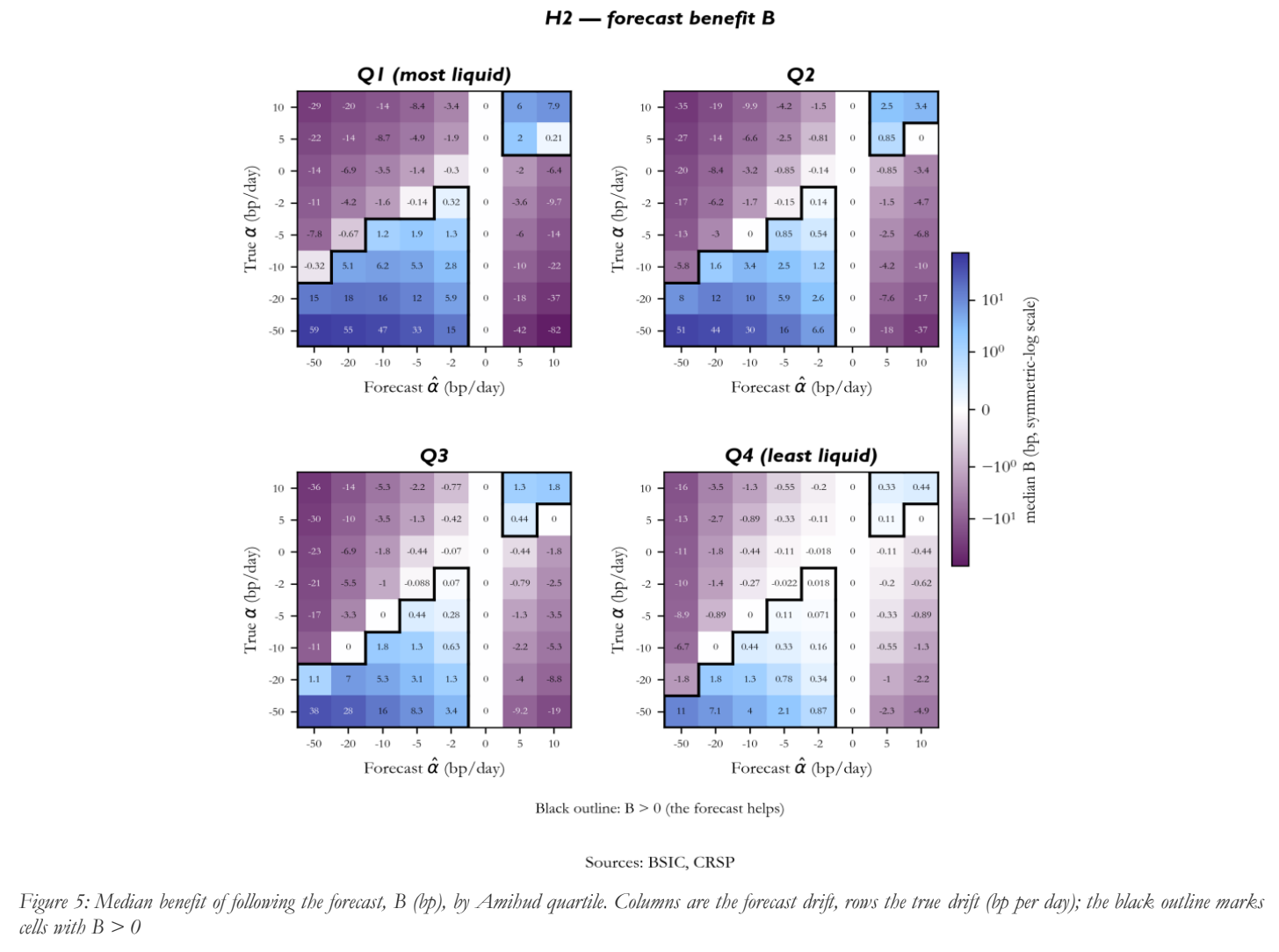
Figure 5 maps the median benefit for every forecast and true drift. Three patterns are common to all quartiles. Forecasts of the right sign and similar size help (the outlined blue region); forecasts of zero change nothing (the white column); and forecasts of the wrong sign hurt, often by more than a correct forecast would have gained. When the true drift is −20bp per day, a forecast of +10bp costs a median 37bp in Q1, more than twice the 17.8bp that a perfect forecast would have earned. The top rows of each panel show the mirror image: when the true drift is positive, the useful forecasts are positive too, and a fund that delays its sales in anticipation of a rising price benefits, while a fund that front-loads on a mistaken expectation of selling pressure loses up to 29bp in Q1 and 36bp in Q3. The loss L, shown in Figure 7, carries the same information from the other side: L is zero on the diagonal, grows with the squared distance from it in the unconstrained cells and is never negative. Wherever the constraint is slack, the size of a cell, positive or negative, falls from Q1 to Q4, as the formula B = G · r(2 − r) predicts: liquidity scales the money at stake in both directions. The exceptions are very strong negative forecasts, where the constraint caps the response of liquid stocks, a point we return to below.

Table 6 isolates the reference truth of −10bp per day. For Q4, where the constraint almost never binds, the median ratio B/G follows r(2 − r) to the third decimal: 0.75 for a forecast of −5bp, 0 for −20bp, −1.25 for +5bp and −15 for −50bp; Q3 does the same except at −50bp. Across all unconstrained stock–pairs the formula matches the numerical solution with a maximum error of 3.5×10⁻⁷. The most liquid quartile behaves differently.

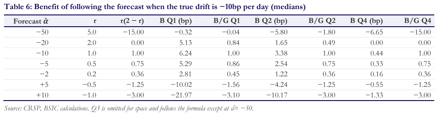
Binding constraints change the rule. For a Q1 stock with a true drift of −10bp, a forecast of −20bp, twice the truth, still delivers 84% of the perfect-forecast gain instead of nothing, and a forecast of −50bp costs 0.3bp instead of fifteen times the gain. The reason is that the non-negative sales constraint caps how far a liquid stock can respond to any negative forecast: once the fund sells nothing on the last days, a more extreme forecast cannot push it further, so overestimation is cheap. The constraint binds for 85% of Q1 stocks already at a forecast of −10bp, against none in Q4, and only 21.5% of the Q1 stock–pairs lie in the unconstrained regime, against 94.5% in Q4. For the most liquid stocks the universal rule is therefore the exception rather than the norm.

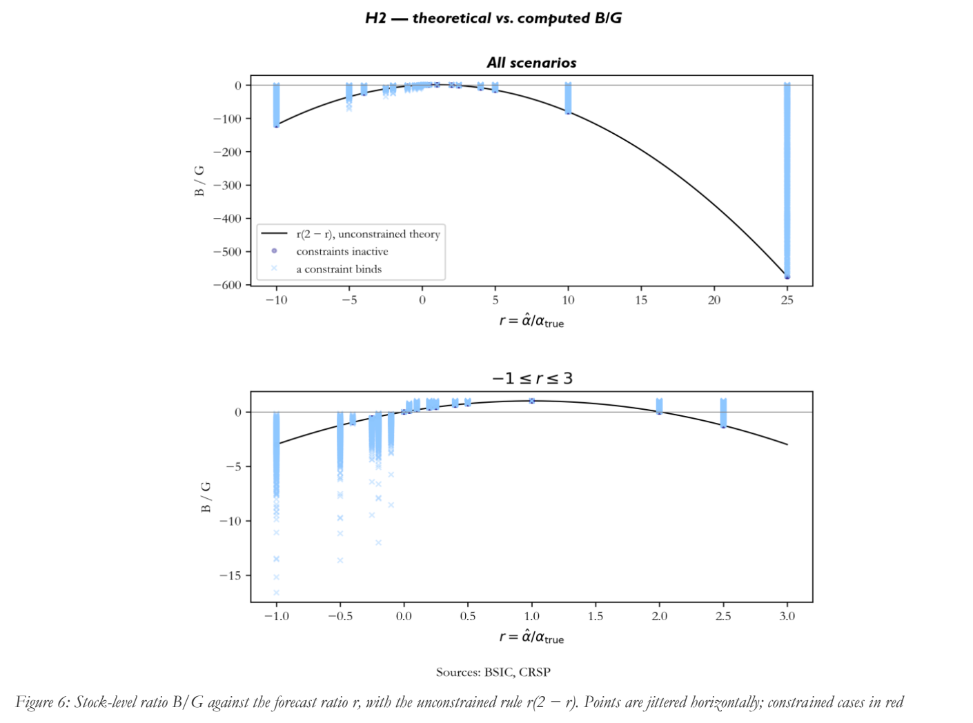
Figure 6 shows the departures across all stocks. Unconstrained cases lie on the parabola to within 3.5×10⁻⁷, so every material departure comes from a pair in which the constraint binds for the forecast or for the true-drift schedule; among constrained pairs other than the trivial cases r = 0 and r = 1, fewer than 0.1% lie within 10⁻⁶ of the parabola. For right-sign forecasts that do not overstate the drift, the sign results above guarantee B ≥ 0: on our grid these are the pairs with 0 < r ≤ 1, and all 22,205 constrained ones have a positive benefit, with B/G at or above r(2 − r). Overstatement is where the constraint changes the answer, and there the results are numerical findings rather than guarantees: all 2,915 constrained pairs with r = 2 still benefit, where the formula predicts zero, and 21.9% of the constrained pairs with r > 2 still benefit, where the formula predicts a loss. The constraint therefore moves the threshold for overestimation upward. Table 7 summarises the constrained cases by forecast ratio.

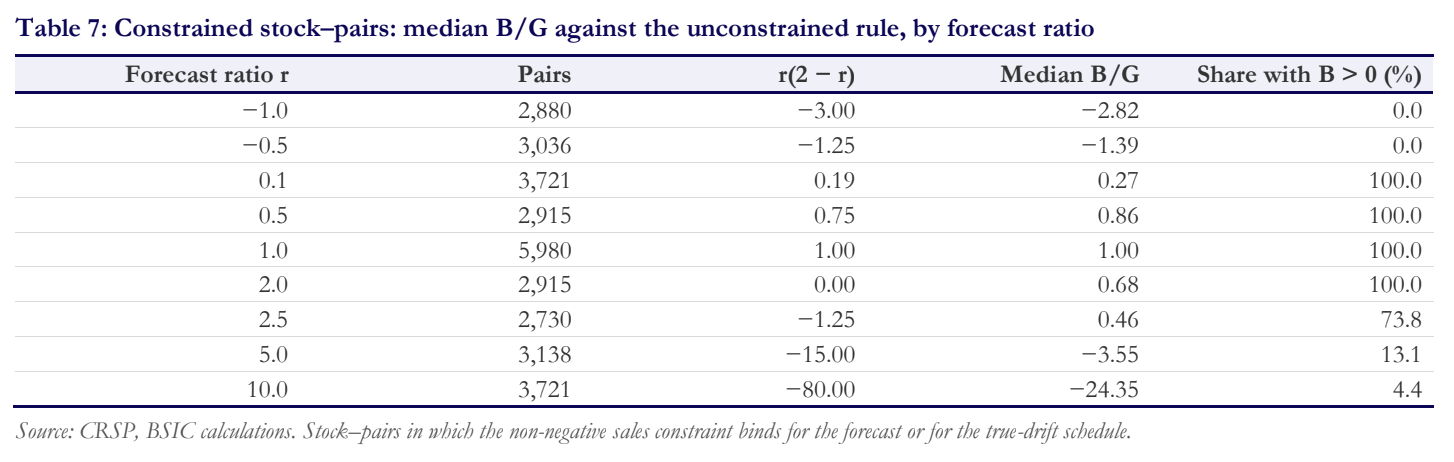
Two features stand out. For forecasts of the right sign up to two and a half times the truth, the median constrained benefit is positive, and at r = 2 it is about two thirds of the perfect-forecast gain rather than zero. Beyond that, the constrained losses are still far smaller than the formula implies: at r = 5 the median ratio is −3.6 instead of −15, and at r = 10 it is −24 instead of −80. The asymmetry is the signature of the constraint: it bounds the schedule’s response to a strong negative forecast, so the damage of overreaction saturates once the sale is completed early. It does not rescue a forecast of the wrong sign: as the sign results guarantee, none of the constrained pairs with r < 0 has a positive benefit, and for small wrong-sign forecasts the constrained losses are slightly larger than the formula’s. Errors in sign remain the costly mistake for every stock.

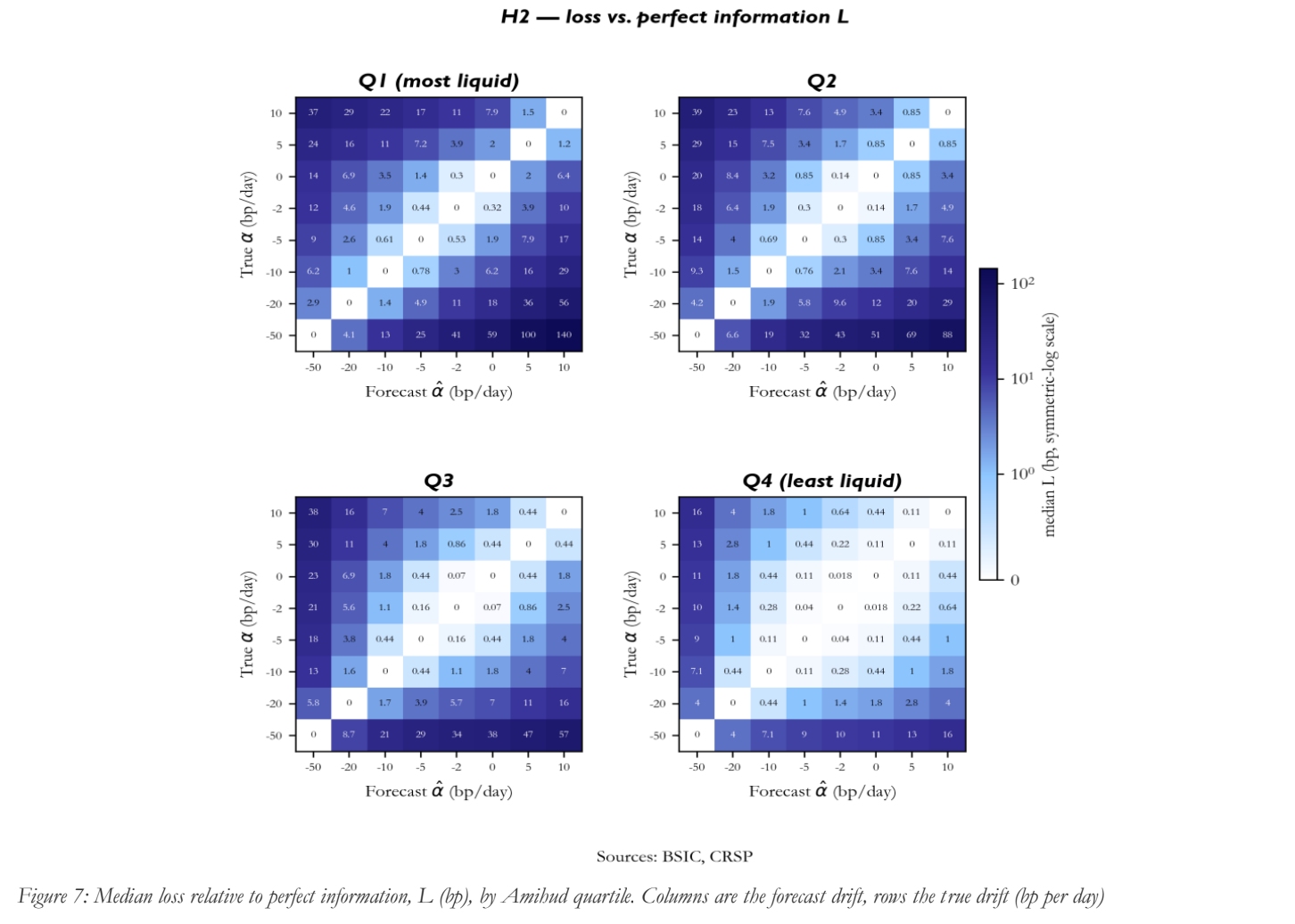
Figure 7 shows the same information from the side of the loss L. The loss is zero on the diagonal, where the forecast is correct, and rises with the distance from it. Its size again falls from Q1 to Q4 for every cell in which the constraint is slack, but for strong negative forecasts the loss in Q1 is smaller than in Q2 and Q3: the constraint protects the most liquid stocks against their own overreaction.

Reading H2. H2 combines three layers that should not be confused. The non-negativity of G and L, the identities linking B, G and L, the sign results for conservative and wrong-sign forecasts, which hold whether or not the constraint binds, and the universal threshold 0 < r < 2 in the unconstrained regime are mathematical implications: they hold by construction and the numerical tests confirm them. The magnitudes of G, B and L, their ranking across quartiles and the frequency and effect of the constraint are calibrated numerical findings: they depend on Almgren and Chriss’s model, the calibration and the hypothetical drifts. The only empirical observations are the inputs, the cross-sectional distribution of spreads, volatilities and volumes, which determine how much each stock has at stake. No realised trading outcome, drift or forecast error is observed.

What This Means for an Execution Desk

Three practical implications follow, with the caveat that they are statements about Almgren and Chriss’s calibrated model rather than about realised trading profits.

Where to spend the forecasting effort. The value of anticipating selling pressure is concentrated in liquid names. For the most liquid quartile a correct forecast of a −10bp drift is worth about a quarter of the cost–risk objective, and the informed and uninformed frontiers visibly separate; for the least liquid quartile it is worth less than half a basis point. A desk with limited research capacity should therefore spend it on the liquid part of its book, which is counter-intuitive: the illiquid names are where execution costs are high, but they are also where little can be done about them by timing.

How to size a forecast. In the unconstrained model the benefit is symmetric around the truth, so understating and overstating the pressure by the same proportion cost the same. The non-negative sales constraint breaks the symmetry in favour of overestimation for liquid stocks: once the schedule completes the sale early, a more extreme forecast cannot make it sell faster. Underestimation, by contrast, is always safe: a forecast with the right sign that does not overstate the drift can never do worse than ignoring it, even when the constraint binds; it simply forgoes part of the gain. For liquid names, a fund that is confident about the direction of the pressure but not about its size loses little by erring on the side of a stronger forecast.

What not to get wrong. A forecast of the wrong sign is harmful for every stock, and the constraint offers no protection: a fund that delays its sales in expectation of a rebound that never comes pays more than it would by ignoring the drift altogether, often more than the whole gain a correct forecast would have delivered. Before acting on a view about other sellers, a desk should therefore be most confident about its direction.

What These Results Do Not Show

The results are conditional on a number of choices, the most important of which are the following.

The drift is hypothetical and exogenous: we do not estimate it, and we do not claim that other investors’ selling necessarily produces a negative drift of any given size. It is also constant and deterministic within the five days, whereas real selling pressure is uncertain, may be concentrated on particular days and may reverse after the sale. Forecast errors are scenarios rather than a distribution: the analysis shows what a given error costs, not how likely it is, and it does not compute an expected benefit under uncertainty about the drift.

The strategy is static. The forecast is fixed at the start and never revised, so the fund does not learn about the drift from prices during the sale, and dynamic strategies are not studied. Other sellers are not modelled strategically, although a fund that anticipates their selling may compete with them to sell first [6], and their selling is assumed to leave the fund’s own temporary impact unchanged, although it may also widen spreads.

Impact is not identified. Daily CRSP data reveal no fund’s orders, so temporary impact comes from Almgren and Chriss’s rule of thumb, it is linear, permanent impact is zero and every cost is proportional to the spread. The closed-form rule requires the constraint to be inactive, which, as we show, is rare among the most liquid stocks. The risk aversion is chosen rather than estimated; G is reported at three levels, but the forecast-error analysis uses only one. The design is fixed at 10% of daily volume sold over five days; both choices affect the level of costs and the value of a forecast, and we do not report other order sizes or horizons. With linear impact the shape of the optimal schedule does not depend on the order size, so very large orders are outside the analysis. Finally, the closing quote is a snapshot rather than the spread paid during the day, Amihud mixes trading frictions with information events, the corporate-action factors are rebuilt from CRSP fields, and all estimates come from a single six-month period. We make no causal claim about Amihud and execution costs.

Conclusion

Almgren and Chriss show that, with independent price increments, known cost parameters and a mean–variance objective, a schedule fixed at the start is optimal, and that a directional view changes it by an amount they find negligible for plausible drifts. Keeping their model and calibration, we asked how stock liquidity and information about anticipated selling pressure shape that schedule for 2,814 US stocks.

H1 is supported without exception. The efficient frontiers of the four Amihud quartiles are perfectly ordered at every common risk level, and the least liquid quartile pays 22 to 27 times more than the most liquid one for the same normalised risk. Part of this is built into a calibration that ties every cost to the spread; the empirical content is that Amihud, which never enters the model, ranks stocks in the same order as the spreads and volatilities that determine their frontiers.

H2 separates the value of correct information from the value of imperfect information. The value of a correct forecast is non-negative by construction; its size is the finding. It is negligible for mild pressure, as Almgren and Chriss concluded, but grows with the square of the drift, reaching a median 41.6bp at −50bp per day, and it is concentrated in liquid stocks, fourteen times larger in the most liquid quartile than in the least liquid at the reference drift. Liquid stocks are cheap to sell, and information about the price matters most for them; illiquid stocks are expensive to sell, and the same information barely changes their schedule.

The value of an imperfect forecast can take either sign. In the unconstrained model it equals the perfect-forecast gain times r(2 − r): a forecast helps if and only if it has the right sign and is less than twice the truth, a threshold that is the same for every stock. That threshold is a property of the quadratic model, not an empirical discovery; what the data determine is the money at stake. Two weaker results hold even when the constraint binds: a forecast with the right sign that does not overstate the drift never hurts, and one with the wrong sign never helps. In practice, the non-negative sales constraint binds for most liquid stocks, and when it does the rule becomes more forgiving: overestimating the pressure costs little, because the fund cannot sell faster than completing the sale early. A wrong sign, by contrast, remains costly for every stock.

For a fund that expects others to sell, the lesson is therefore asymmetric. In liquid names, acting on a forecast of selling pressure is worth a meaningful share of the cost–risk objective, and overestimating it is cheap; getting the direction wrong is not. In illiquid names, the forecast barely matters, because the cost of selling faster outweighs the price it avoids. All of these conclusions are conditional on the data, the sample period, the hypothetical drifts and the execution model assumed.

References

[1] Almgren, Robert, and Neil Chriss, “Optimal Execution of Portfolio Transactions”, Journal of Risk 3(2), 2000, pp. 5–39

[2] Almgren, Robert, “Optimal Execution with Nonlinear Impact Functions and Trading-Enhanced Risk”, Applied Mathematical Finance 10(1), 2003, pp. 1–18

[3] Almgren, Robert, Chee Thum, Emmanuel Hauptmann, and Hong Li, “Direct Estimation of Equity Market Impact”, Risk 18(7), 2005, pp. 58–62

[4] Amihud, Yakov, “Illiquidity and Stock Returns: Cross-Section and Time-Series Effects”, Journal of Financial Markets 5(1), 2002, pp. 31–56

[5] Bertsimas, Dimitris, and Andrew W. Lo, “Optimal Control of Execution Costs”, Journal of Financial Markets 1(1), 1998, pp. 1–50

[6] Brunnermeier, Markus K., and Lasse Heje Pedersen, “Predatory Trading”, Journal of Finance 60(4), 2005, pp. 1825–1863

[7] Carlin, Bruce Ian, Miguel Sousa Lobo, and S. Viswanathan, “Episodic Liquidity Crises: Cooperative and Predatory Trading”, Journal of Finance 62(5), 2007, pp. 2235–2274

[8] Cartea, Álvaro, Sebastian Jaimungal, and José Penalva, Algorithmic and High-Frequency Trading, Cambridge University Press, 2015

[9] Coval, Joshua, and Erik Stafford, “Asset Fire Sales (and Purchases) in Equity Markets”, Journal of Financial Economics 86(2), 2007, pp. 479–512

[10] Gatheral, Jim, “No-Dynamic-Arbitrage and Market Impact”, Quantitative Finance 10(7), 2010, pp. 749–759

[11] Harris, Lawrence, and Eitan Gurel, “Price and Volume Effects Associated with Changes in the S&P 500 List: New Evidence for the Existence of Price Pressures”, Journal of Finance 41(4), 1986, pp. 815–829

[12] Lorenz, Julian, and Robert Almgren, “Mean–Variance Optimal Adaptive Execution”, Applied Mathematical Finance 18(5), 2011, pp. 395–422

[13] Obizhaeva, Anna A., and Jiang Wang, “Optimal Trading Strategy and Supply/Demand Dynamics”, Journal of Financial Markets 16(1), 2013, pp. 1–32

[14] Perold, André F., “The Implementation Shortfall: Paper versus Reality”, Journal of Portfolio Management 14(3), 1988, pp. 4–9

[15] Shleifer, Andrei, “Do Demand Curves for Stocks Slope Down?”, Journal of Finance 41(3), 1986, pp. 579–590

[16] Center for Research in Security Prices (CRSP), “CRSP US Stock Database (CIZ format), daily stock file”, accessed through Wharton Research Data Services, 2025