Do Norges Bank’s Announced FX Transactions Contain Incremental Information About NOK Exchange Rate Dynamics?

Download PDF

Introduction

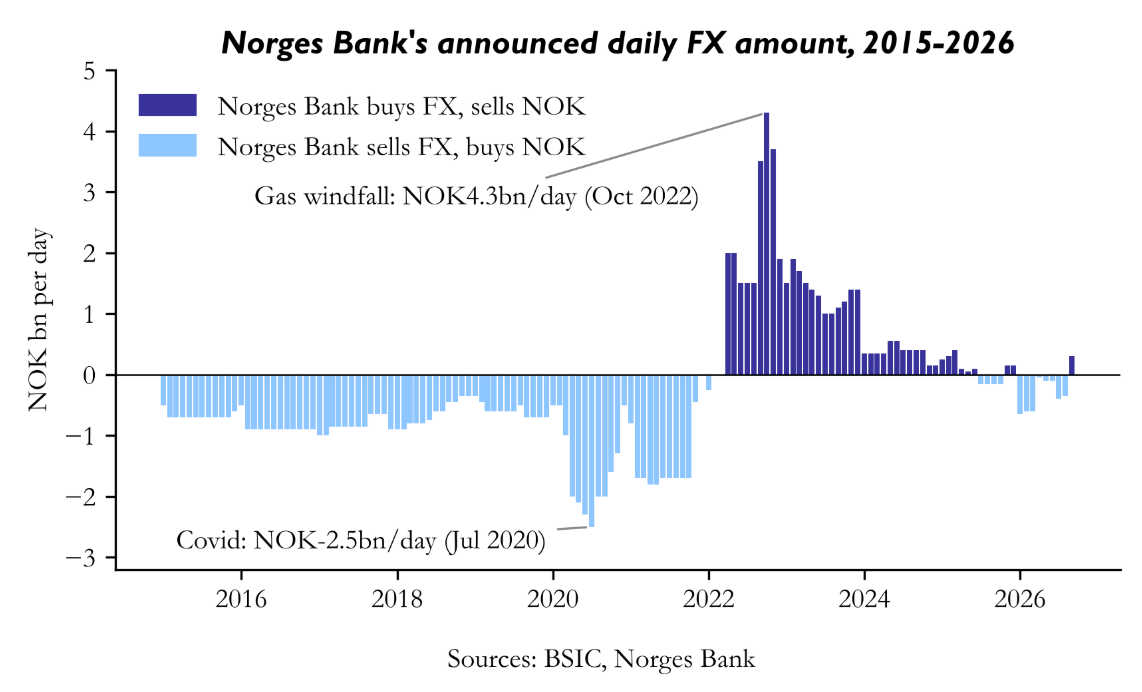
Every month, Norges Bank tells the market exactly how much foreign currency it will buy or sell on behalf of the Norwegian government over the following month. At their peak in October 2022 these transactions reached NOK4.3bn per business day, a very large and fully pre-announced flow for a currency market of the krone’s size. A large literature on currency order flow finds that who buys and sells a currency helps explain how its price moves. Norges Bank’s transactions therefore offer an unusually clean experiment: a very large flow, executed mechanically, whose size is public a month in advance.

This article asks whether those announcements contain incremental information about EUR/NOK, meaning information that is not already explained by the usual drivers of the krone: oil prices, global risk sentiment and the interest-rate differential with the euro area. We test three channels. First, does the krone react when the new monthly amount is published? Second, does it move on the days Norges Bank actually trades? Third, can the announced amount be used to forecast next month’s EUR/NOK return?

The answer is precise. The krone reacts on the announcement day: across 143 announcements between 2015 and 2026, a NOK1bn increase in the announced daily FX purchase weakens the krone by about 0.41% against the euro on the day of the release (p = 0.004). After that, nothing. The execution flow has no measurable effect, the announcement-day move partly reverses the next day, and the announced amount does not beat a random walk out of sample. In the language of market efficiency, the information is priced on the day it becomes public, and not after.

Why This Matters Now

The government’s FX transactions have swung from one extreme to the other in the past six years. In 2020, Norges Bank sold up to NOK2.5bn of foreign currency per day to fund the pandemic budget deficit. In 2022, the gas-price windfall reversed the flow, and Norges Bank bought up to NOK4.3bn per day. Since 2024 the amounts have been much smaller, and since mid-2025 they have changed sign several times, from selling NOK650m per day in January 2026 to buying NOK300m per day in September and October 2026.

For anyone trading NOK, the question is whether these announcements are a tradable signal or simply noise that the market absorbs immediately. The answer also matters for policy: Norges Bank designs the transactions to be predictable precisely so that they do not disturb the krone. If they still moved the currency after being announced, that design would not be working.

The Mechanics of Norges Bank’s FX Transactions

The Norwegian government receives petroleum revenue both in kroner and in foreign currency, and part of that revenue is used to finance the planned central government budget deficit. Norges Bank carries out the foreign exchange transactions this requires. When the government needs more kroner than its petroleum revenue provides, Norges Bank sells foreign currency; when petroleum revenue in foreign currency is high, as in 2022, it buys foreign currency for transfer to the Government Pension Fund Global.

▪  Announcement. On the last business day of each month, Norges Bank publishes the amount it will trade on each business day of the following month. The release is published at 10:00 Oslo time (verified for the January 2026 release), before the 14:15 CET fixing used in this article.

▪  Execution. The same amount is traded on every business day of that month. Mid-month changes are rare: there have been five since 2000, three of them inside our sample (18 March 2020, 23 November 2020 and 18 November 2021).

▪  Sign. A positive amount means Norges Bank buys foreign currency and sells kroner, which in principle weakens the krone. A negative amount means it sells foreign currency and buys kroner, which in principle supports it.

Because the amount is published in advance, an efficient market should price it on the announcement day. If the krone still moved with the flow on the days it is executed, or if the announced amount predicted later returns, the announcements would contain information that the market fails to use.

Data

The sample runs from 5 January 2015 to 30 September 2026: 2,955 Norges Bank business days, 140 complete months and 143 announcements. All series are aligned to the Norges Bank business-day calendar.

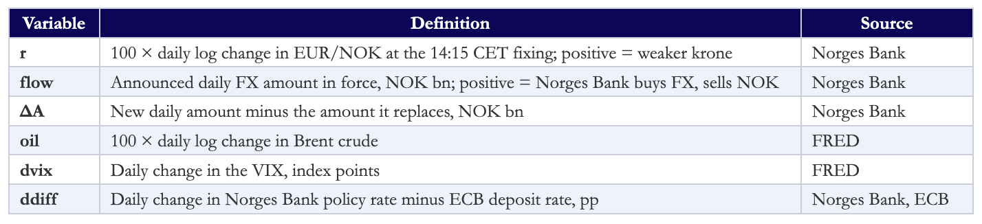
The announcement series is taken from Norges Bank’s data API rather than the table on its website. The website shows a single figure per month and, for March and November 2020, reports the amount that applied after the mid-month change as if it applied to the whole month; the API records each announcement with its exact effective date. Brent and the VIX are not quoted on 34 and 46 Norges Bank business days respectively (US and UK holidays). On those days the last available close is carried forward, so their daily change is zero.

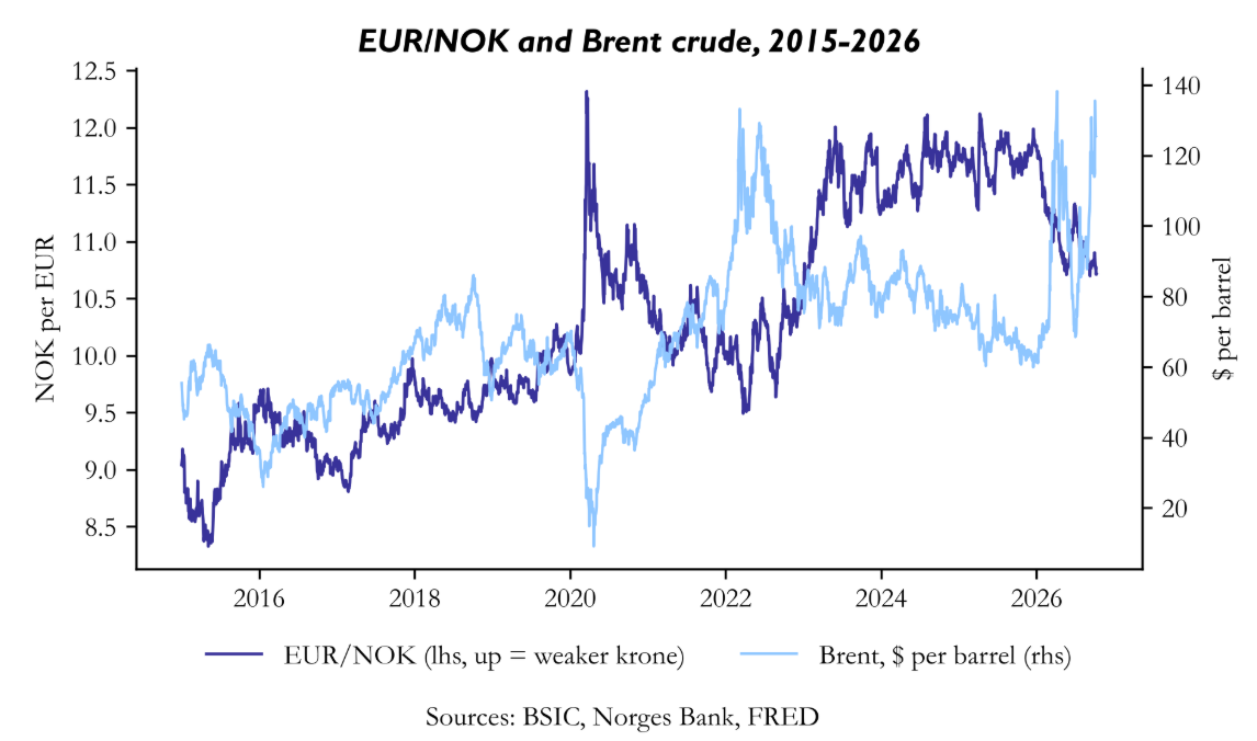
The chart illustrates why oil must be controlled for. The krone weakened sharply when Brent collapsed in 2020, and its broad level over the decade moves with the oil price and with global risk appetite. A naive comparison of the flow with EUR/NOK would therefore risk crediting Norges Bank with moves that oil or risk sentiment caused.

Econometrics Toolkit: From Returns to p-values

Before turning to the tests, we explain each tool from first principles. Readers familiar with regression analysis can skip to the methodology.

Step 1 – Measuring a move: log returns

EUR/NOK is the number of kroner needed to buy one euro, so an increase means a weaker krone. We measure daily moves with log returns, expressed in percent:

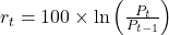
If EUR/NOK moves from 11.50 to 11.55, the log return is 100 × ln(11.55/11.50) = 0.434%, almost identical to the simple percentage change. Log returns are used because they add up over time, so the return over a window of days a to b is simply the sum of the daily returns:

Step 2 – Linking two variables: linear regression

A regression measures how much one variable moves on average when another moves, holding everything else in the model fixed. With one explanatory variable x:

Here α is the constant, β is the slope we care about (the average change in y for a one-unit change in x) and ε captures everything else. Ordinary least squares (OLS) picks the α and β that minimise the sum of squared errors. With one regressor the solution is the covariance of x and y divided by the variance of x; with several regressors stacked in a matrix X, it is:

Because the krone also moves for reasons unrelated to Norges Bank, every regression includes three control variables: the Brent return (a higher oil price tends to strengthen the krone), the change in the VIX (global stress tends to weaken it) and the change in the policy-rate differential. β then measures the effect of the flow holding oil, risk sentiment and rates fixed. R², the share of the variation in y explained by the model, summarises the fit:

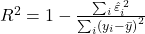
Daily currency returns are dominated by noise, so an R² of around 0.10 is typical for daily FX regressions.

Step 3 – Is the effect real? Standard errors, t-statistics and p-values

An estimated β is never exactly the true effect, because it comes from a limited and noisy sample. The standard error (SE) measures how precisely β is estimated. The t-statistic counts how many standard errors the estimate lies away from zero, and the p-value converts it into a probability:

The p-value is the probability of finding an estimate at least this far from zero if the true effect were zero (the null hypothesis, H0: β = 0). We use 5% as the conventional threshold. Two points matter for reading the results. A p-value is not the probability that the effect is real, and a large p-value means the data cannot distinguish the effect from zero, not that the effect has been proven to be zero. Equivalently, a 95% confidence interval collects the values of β that the data cannot reject:

Financial data violate the textbook assumptions behind the simplest SE formula, so we use robust versions. HC1 standard errors allow the size of errors to differ across observations; this matters because EUR/NOK was far more volatile in March 2020 than in 2017. Standard errors clustered by month allow errors to be correlated within a month, which matters because the flow is identical on every day of a month. Newey-West standard errors allow errors to be correlated with those of the previous few periods.

Step 4 – Event studies, surprises and permutation tests

An event study looks at prices in a fixed window around a known event. Day 0 is the announcement day, day -1 the day before and day +1 the day after. Averaging across many events cancels unrelated news and leaves the typical reaction. A placebo test repeats the exercise on a window where no effect should exist, such as day -1. Markets react only to the unexpected part of an announcement, the surprise:

Finally, a permutation test checks significance without relying on any distributional formula. The announced changes are randomly shuffled across announcement days, which breaks any genuine link with returns, and β is re-estimated. Repeating this S = 10,000 times shows how large β becomes by chance alone; 1(·) equals one when the condition inside holds and zero otherwise:

Step 5 – In-sample is not out-of-sample

A model can always fit the past by chance. Out-of-sample testing mimics a real investor: each month the model is estimated only on data available at the time and then used to forecast the next month. Forecasts are scored against a benchmark with the out-of-sample R²:

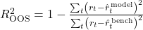
A positive value means the model beats the benchmark. The toughest benchmark in currencies is the random walk, which forecasts a return of zero every month; beating it is famously difficult. Because our model nests its benchmark, we test the difference with the Clark-West statistic, which corrects for the noise introduced by estimating extra coefficients:

where model 0 is the benchmark and model 1 adds the flow. Regressing f on a constant gives the test statistic.

Methodology

The three tests examine the same flow at three moments: when it is announced, while it is executed, and before the month begins.

Test 1 – The announcement effect

For each announcement i with event day t, the cumulative EUR/NOK return over the window [a, b] is regressed on the change in the announced daily amount:

If β is positive and significant, larger increases in Norges Bank’s NOK selling coincide with a weaker krone. We use the windows [0], [0,+1], [-1,+1] and [+2,+10], the placebo [-1] and the next day [+1], with HC1 standard errors. Two surprise measures are used: the raw change ΔA, which assumes the market expected no change, and the residual from a real-time model that predicts ΔA from the previous month’s Brent and EUR/NOK returns and the current amount, estimated only on earlier announcements. The rate differential drops out of the short windows because no policy rate changed on an announcement day.

Test 2 – The execution effect

Each daily return is regressed on the amount traded that day:

Because the flow is public in advance, an efficient market implies β = 0. Standard errors are clustered by month (141 clusters), with Newey-West (5 lags) as a check. Re-running the test without the 143 announcement days ensures the result reflects execution rather than the announcement reaction.

Test 3 – Monthly explanatory and predictive regressions

Monthly returns R are regressed on F, the business-day average of the announced daily amount, first with controls from the same month and then with information available only at the start of the month:

Newey-West standard errors with 3 lags are used. The first equation asks whether the flow explains anything once oil, risk and rates are accounted for; the second asks whether an investor at the start of the month could have used it to predict the month’s move.

Test 4 – Out-of-sample forecasts and reverse causality

Expanding-window forecasts of the monthly return start in February 2020 (80 months) after a 60-month initial window. The model with the flow is compared with lagged controls alone and with a random walk. Finally, the change in next month’s announced amount is regressed on this month’s EUR/NOK and Brent returns, to check whether the amount itself responds to the krone.

Results: The Krone Reacts on the Day, and Only on the Day

The change in the announced amount is significant on the announcement day and in no other window. A NOK1bn increase weakens the krone by 0.41% (p = 0.004). The typical non-zero change is NOK0.2bn, which implies a typical move of about 0.08%; a one-standard-deviation change of NOK0.4bn implies about 0.16%.

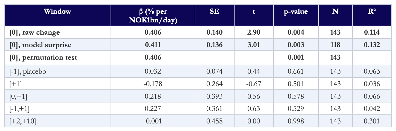
All regressions control for Brent and the VIX over the same window and use HC1 standard errors. The permutation test confirms the result without any distributional assumption: only 13 of 10,000 random shuffles produced a coefficient as large as the actual one. The placebo on the day before the announcement is flat, which rules out leakage and pre-positioning.

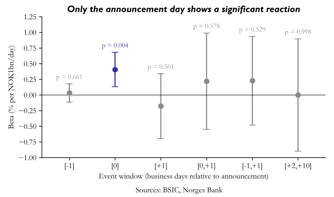
The [+1] coefficient is negative (-0.178), so part of the day-0 move tends to reverse the following day, although that reversal is not significant on its own (p = 0.50). It is enough, however, that the [0,+1] window is no longer significant (p = 0.58). The event-study paths below tell the same story: increases in the amount are followed by a 0.22% weakening on day 0, with a 95% confidence interval of 0.06% to 0.38%, after which the bands widen and include zero.

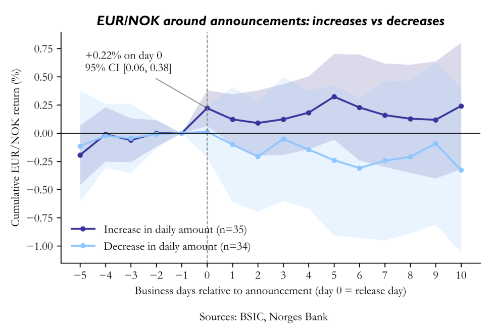
The reaction is directional, not a volatility effect. Absolute EUR/NOK returns average 0.359% on announcement days against 0.392% on other days (Welch t-test p = 0.31, Mann-Whitney p = 0.052). If anything, announcement days are slightly calmer: the market reacts to the direction of the change, not to the event itself.

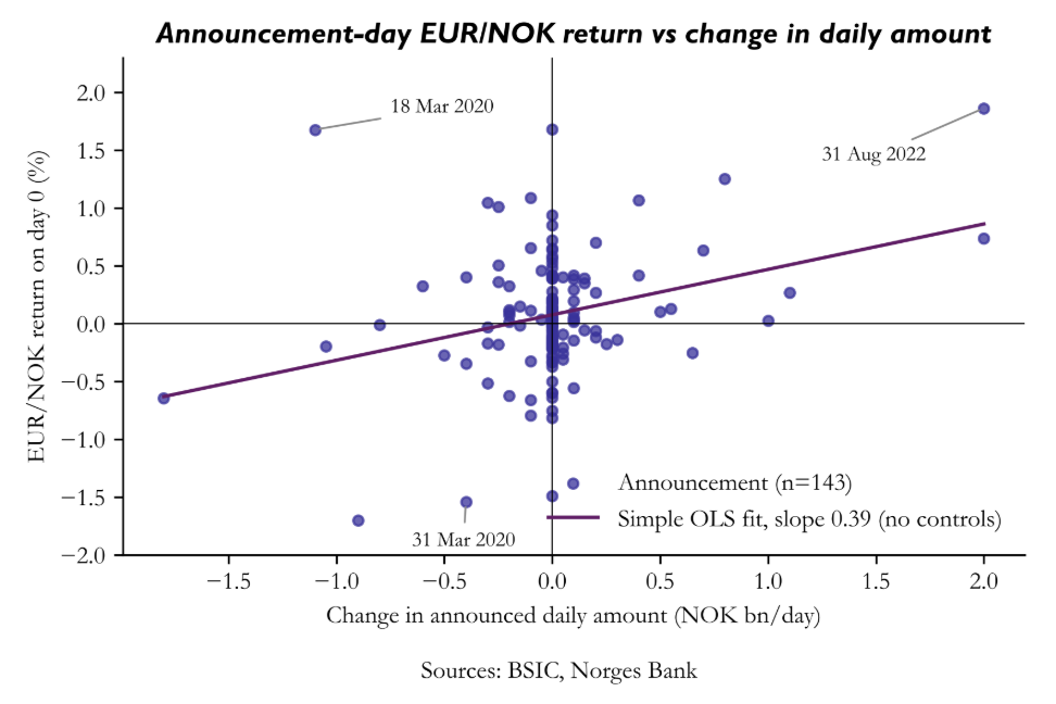
The scatter shows both the relation and its fragility. Most announcements leave the amount unchanged or change it by less than NOK0.5bn, and the slope is anchored by a handful of large changes, notably 31 August 2022, when Norges Bank raised its daily purchases by NOK2.0bn and EUR/NOK rose 1.86% on the day.

Execution Does Not Move the Krone

Once the amount is public, the daily flow has no measurable effect. Oil and global risk carry the explanatory power.

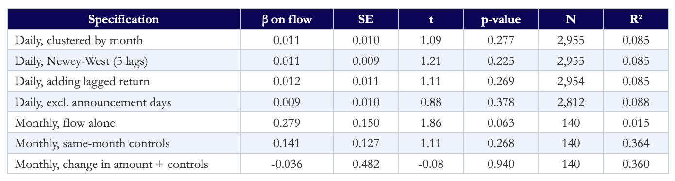
A coefficient of 0.011 implies that even at the 2022 peak of NOK4.3bn per day the krone would be only about 0.05% weaker per day, and that estimate cannot be distinguished from zero (p = 0.28). The controls behave as expected: a 1% rise in Brent strengthens the krone by 0.037% and a one-point rise in the VIX weakens it by 0.047% (both p < 0.001). At monthly frequency, the flow alone looks borderline (p = 0.063), but the effect disappears once oil, the VIX and rates are added (p = 0.27). Controls alone explain 36.0% of monthly variance; adding the flow lifts R² only to 36.4% (Wald test p = 0.27). The flow was picking up oil and risk moves that happened at the same time.

The Announced Amount Does Not Forecast the Krone

In-sample, the amount known at the start of the month appears marginally significant for that month’s return (β = 0.338, SE 0.167, p = 0.043.

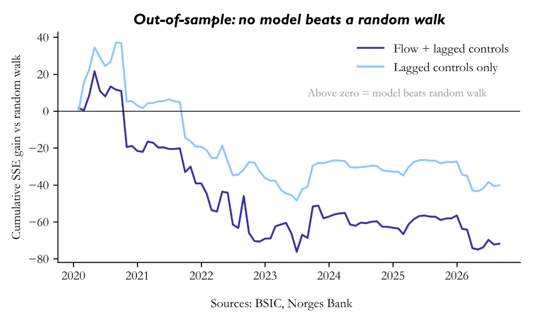
A negative out-of-sample R² means that forecasting “no change” every month would have produced smaller errors. The cumulative error lines fall below zero during 2020 and never recover, and adding the flow makes the forecasts worse rather than better. The in-sample p-value of 0.043 is therefore most plausibly a fitting accident, which is precisely what out-of-sample testing is designed to expose.

Reverse causality does not drive the results either. The change in next month’s announced amount is unrelated to this month’s EUR/NOK return (β = 0.006, p = 0.73) or Brent return (β = 0.004, p = 0.14), with R² = 0.050. Our real-time model explains only 3.1% of announced changes, so with public market data the announcements are close to unpredictable.

Robustness: How Fragile Is the Announcement Effect?

The day-0 effect survives most checks, but it leans on 2022. Dropping the 2022 events in addition to 2020 cuts the coefficient to 0.32 and the p-value to 0.19, R² = 0.067, N = 140, controlling for the lagged return, Brent, VIX and rate differential). Out of sample, the signal fails.

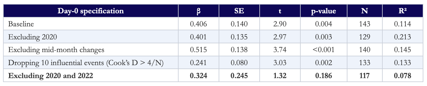
Influential events are identified with Cook’s distance, which measures how much the fitted values change when one observation is removed; the usual rule flags observations with D > 4/N. The two most influential events are 31 March and 18 March 2020, both during the pandemic collapse of the krone. The monthly flow coefficient is insignificant in every subsample: 2015 to 2019 (β = 1.04, p = 0.37, N = 59), 2020 to 2026 (β = 0.18, p = 0.19, N = 81) and excluding 2020 (β = 0.16, p = 0.29, N = 128).

Because we estimate eight event windows, we also correct for multiple testing. The Bonferroni correction multiplies each p-value by the number of tests, m:

The day-0 p-value of 0.004 survives (adjusted p = 0.03), while the in-sample predictive p-value of 0.043 does not survive any correction.

What Would Change This Conclusion?

Several limitations should be kept in mind. First, the market’s true expectation of each announcement is built from the Ministry of Finance’s budget and petroleum-revenue estimates, which we do not use. Our raw change therefore overstates the true surprise, which biases β toward zero rather than away from it. Second, returns are measured between 14:15 CET fixings; intraday data around the 10:00 release would isolate the reaction and remove unrelated news. The release time was verified on the January 2026 announcement and assumed for earlier releases. Third, Norges Bank also buys kroner to fund its own dividend transfer to the government, for example NOK126m per day from March 2025 to February 2026, and that flow is not part of the series used here.

Finally, regular announcements fall on the last business day of the month, when the krone also experiences month-end rebalancing flows. The constant in the day-0 regression (0.07%, p = 0.064) absorbs the average month-end move, but the flow coefficient would be biased if month-end flows were correlated with the announced change. Evidence of a persistent execution effect, or a positive out-of-sample R² using budget-based surprises, would overturn our conclusion.

Conclusion

Norges Bank’s announcements contain information that the market prices immediately, and none that it prices late. The krone moves on the announcement day in the direction the flow implies, by about 0.41% per NOK1bn of daily change. After that, the executed flow has no detectable effect, and the announced amount does not forecast monthly EUR/NOK returns out of sample.

The evidence fits a market that treats the flow as known information rather than as ongoing price pressure, which is exactly what Norges Bank’s transparent design aims for. For traders, the only potentially usable window is the few hours between the 10:00 release and the 14:15 fixing, and even that effect rests heavily on a few large changes in 2020 and 2022. The natural next step is to test that window with intraday EUR/NOK data and to measure surprises against the Ministry of Finance’s budget-based estimates.

References

[1] Norges Bank, “Foreign exchange transactions on behalf of the government,” statistics.

[2] Norges Bank, Data API, dataset ANN_FX_SPU, “Announcement of foreign exchange transactions on behalf of SPU,” 2000 to 2026.

[3] Norges Bank, Data API, dataset EXR, “Exchange rates,” EUR/NOK daily fixing.

[4] Norges Bank, Data API, dataset IR, “Policy rate,”.

[5] European Central Bank, ECB Data Portal, series FM.B.U2.EUR.4F.KR.DFR.LEV, “Deposit facility rate,”.

[6] Federal Reserve Bank of St. Louis, FRED, series DCOILBRENTEU, “Crude Oil Prices: Brent – Europe,”.

[7] Federal Reserve Bank of St. Louis, FRED, series VIXCLS, “CBOE Volatility Index: VIX,”.

[8] Norges Bank, press release on foreign exchange transactions for the government in February 2026, published 30 January 2026.

[9] Meese, Richard A.; and Rogoff, Kenneth, “Empirical Exchange Rate Models of the Seventies: Do They Fit Out of Sample?,” Journal of International Economics 14(1-2), 1983, pp. 3-24.

[10] Clark, Todd E.; and West, Kenneth D., “Approximately Normal Tests for Equal Predictive Accuracy in Nested Models,” Journal of Econometrics 138(1), 2007, pp. 291-311.

[11] Newey, Whitney K.; and West, Kenneth D., “A Simple, Positive Semi-Definite, Heteroskedasticity and Autocorrelation Consistent Covariance Matrix,” Econometrica 55(3), 1987, pp. 703-708.

[12] Cook, R. Dennis, “Detection of Influential Observation in Linear Regression,” Technometrics 19(1), 1977, pp. 15-18.

[13] MacKinlay, A. Craig, “Event Studies in Economics and Finance,” Journal of Economic Literature 35(1), 1997, pp. 13-39.

[14] Evans, Martin D. D.; and Lyons, Richard K., “Order Flow and Exchange Rate Dynamics,” Journal of Political Economy 110(1), 2002, pp. 170-180.

[15] White, Halbert, “A Heteroskedasticity-Consistent Covariance Matrix Estimator and a Direct Test for Heteroskedasticity,” Econometrica 48(4), 1980, pp. 817-838.