It is probably fair to say that central banks have become the most powerful actors in today’s financial markets. On the one hand this is due to governments’ reluctance to make use of fiscal policy measures in order to stimulate their economies in the aftermath of the Great Recession. On the other hand their importance also rose in connection with their discovery of unconventional policy tools such as Quantitative Easing (QE).
Instead of acting in tandem, however, the policy stance of two of the most influential institutions is expected to diverge further over the next few weeks. The US Federal Reserve which ended QE already in late 2014 and dared to hike interest rates for the first time in almost a decade last December, is weighing economic conditions in the world’s largest economy for further increases. On the contrary, ECB president Mario Draghi is seen to drive rates in the opposite direction and to ramp up the institution’s bond-buying program. Though both central bank governors attempt to act within their political mandate, repercussions of these diverging actions will impact financial markets as no orderly mechanism exists to manage them. Hence, it is of crucial importance to understand what is guiding central bankers in their decisions and, especially in the case of the Fed and the ECB, what are the underlying considerations for their divergence.
Unlike the Federal Reserve in U.S., the European Central Bank presents only a single mandate, which is prices stability. This concretizes into a targeted medium term goal of inflation “close but below 2%”.
As shown in the chart above, inflation estimates for 1-year and 2-years ahead, it is possible to notice a persistent overestimation trend with respect to the 2-years expectations, which, on one hand, raises questions on the effective achievability of the medium term target, but on the other hand it poses no doubts on the ability of the ECB to be nonetheless credible.
A question that could remain unresolved following a comparison with the Fed rule guiding monetary policy decisions, is why the ECB doesn’t put great emphasis on the output gap when decisions are made.
The main reason has to do with a problem of data; in fact we can observe an extreme unreliability of real time estimates of the output gap in the Euro area.
This might be partially related to the fact that the Euro area is composed by single states using different methods of data collection; due to this, harmonization might not be easy and it might require time, thus distorting real time data.
However, this really poses a problem and several examples can be made on how this could have led the ECB to a wrong monetary policy decision.
The discrepancy between real time and retrospective output gap estimates is well summarized by the figure above, where the thick black line represents the historical output gap estimates published by the European Commission in fall 2011. The dashed lines, instead, show the real time output gap estimates of the year from the European Commission fall and spring forecasts of each quarter in each year.
Looking at the 2006 estimate we can see that if the ECB had set its monetary policy according to the real time estimate of the output gap, it would have adopted a loosening stance, which, in light of data revision, would have been a terrible mistake.
In fact in 2006 the output gap was actually substantially positive and the economy was, if anything, overheated at that time. Same thing applies to 2007 when the turmoil in financial markets started.
Another difference with the Fed, more theoretical than practical, relates to the attitude of the ECB towards the overnight market rate; unlike the Fed, that officially targets the market federal funds rate, the ECB (in the same way as Bank of England) doesn’t officially target any market rate, however EONIA is the market rate that the ECB aims at targeting when setting the Main Refinancing Rate. In light of what previously said, it is thus easy to understand why the Taylor rule is not appropriate for approximating the ECB’s interest rate decisions. The Orphanides-Wieland rule is instead the one adopted as guideline.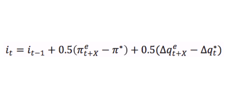
Given that monetary policy isn’t instantaneous in its effects, which means that it operates with a time lag, decisions taken today should be based on the expectations of the future.
represents the expected inflation at the time the decision is taken for t+X.
X is not defined as there is a degree of discretion on the “near-term” horizon that should be adopted, however we will use the 1 year horizon for our estimation.
is the inflation target, is the expected output growth at time t for t+X and is the real time potential output growth.
As we can see no output gap appears here, rather the output growth is used: the reason is mainly mathematical as large mistakes in the output gap result just in minor digit points variations in growth terms, thus solving the problem of real time unreliability.
In the chart, it is possible to see the results of the application of the Orphanides-Wieland rule with a one-year horizon, using SPF surveys for expected inflation and output growth and European Commission’s estimates for potential output growth. The bounds are also estimated: the lower one with an inflation goal of 2% and the upper one with an inflation goal of 1.5%.
As it is possible to see, in the most part of cases, the main refinancing rate lies in the middle of the estimation corridor or really near to one of the bounds, mostly the 2% bound.
The only case where there is a huge difference between the OW rule prescription and the actual interest rate adopted is between 2009 and 2011 when the ECB adopted other unconventional monetary policy tools to deal with the economic situation, which aren’t embedded into the main refinancing rate level.
Furthermore, an analysis of the rules guiding monetary policy is not interesting just to study historical decisions and data but also to get some forecasts regarding future monetary policy decisions as the chart above shows.
In conclusion, the different political mandates and underlying rate-setting models of the Fed and the ECB can in part explain their diverging actions. Moreover, they help to better understand the varying post-crisis management of the two institutions. Taking the output gap into consideration, the Fed reacted more aggressively and initially pursued a looser monetary policy than its European counterpart. Given the above-mentioned unreliability of real-time economic data in Europe, this seems plausible. However, it also makes a case for increased attention to economic output in the political decision process of the ECB in alternative forms, effectively adjusting closer to the Fed’s approach. According to economic data, the US seems in a much more robust shape than Europe where several member states still struggle to return to pre-crisis GDP per capita levels.
Moreover, trying to understand central bankers will also bode well for investors who can adjust their asset allocation accordingly. As a word of caution, though, as shown above, any unconventional measures can severely impact the accuracy of the Orphanides-Wieland forecast. Given the expectation of an extension of QE in the Eurozone, market participants should hence tread carefully in making their decisions.
[edmc id= 3529]Download as PDF[/edmc]


0 Comments