Stock Prices Forecasting with Machine Learning

Download PDF

Introduction

Stock prices forecasting is a deeply researched topic, which has been enhanced by the use of Machine Learning techniques since the late 90s. In this article, we present the main methods and models employed by the current literature, along with our own proprietary model.

Literature Review

Over the past 25 years, various applications of Machine Learning to stock prices forecasting have been proposed. Due to its learning nature, Machine Learning is a popular tool to identify stock trends by working with big data. For instance, some papers assessed the predictive power of news articles (Nikfarjam A. et al., 2010), while others focused on the impact of stock earnings announcements (Khanal et al., 2017). Among the most employed techniques are linear regression, logistic regression, k-NN, neural networks and, most prominently, support vector machines (SVM). The features of such models are usually derived from technical indicators, financial ratios, macroeconomic data, or news data. Recently, stock chart images have been adopted directly as an input to study the behavior of prices (Kelly et al., 2020).

As shown by Day and Zhang (2013), short term predictions are not accurate since the current stock price incorporates all publicly available information due to the market’s efficiency, while long term predictions can significantly outperform the underlying stock performance. This is also confirmed by Basaka (2018), which uses technical indicators and tree-based classifiers to predict stock prices. The results demonstrate that a longer trading window increases the accuracy of the machine learning method. On the other hand, when observing a shorter trading window, the success of the prediction of the model was close to random when using XGBoost. Still, when trying to predict the price of AAPL stock in a 90-day trading window, they obtained an AUC score of 0.86. Results obtained by Ariyo (2014) demonstrate that when using the ARIMA statistical method, shorter timeframe predictions are more accurate.

Data Sources

We built a model that classifies SPY returns on two different time frequencies: day, and hour. The dataset is obtained through alphavantage.com for the intraday data, and it spans a period of 2 years, from November 2020 to November 2022. For the daily data instead, we use the WRDS CRSP dataset, which spans 22 years of time, from January 2000 to March 2022. For each data point, we have the open, close, high, low, and volume levels of the SPY. The number of rows depends on the time frequencies, which range from 8,000 to 413,000.

Models

We decided to test two classification models, the logistic regression and XGBoost. Logistic regression is similar to linear regression, but instead of predicting a continuous variable, it predicts the truth of a binary variable. Mathematically, instead of fitting a line to the data, logistic regression fits an S-shaped “logistic function”, which goes from 0 to 1 with 1 being the true, and 0 being the false statement. The value of the logistic function should be interpreted as the probability that the statement is true for a certain datapoint. Despite this, logistic regression is usually used as a classification model, and a threshold is set up, such that the statement is considered true for all of the data points with score above , and false for all of the data points that are below it. In order to calculate the function, the odds on the y-axis are turned into log-odds that go from negative infinity to infinity, through the logit function:

Then, a line is fit to the data using the maximum-likelihood method. The data points or projected on the line, and using this data the log-odds are transformed into normal odds using:

,

where stands for the intercept of the line, b refers to the slope, and x is the input value.

XGBoost stands for “Extreme Gradient Boost”, it is a more scalable and efficient version of the gradient boost algorithm that is suitable for classification and regression. The result is produced by an ensemble of decision trees, which aim to reduce a loss function. Several regularization parameters are employed in order to mitigate overfitting. XGBoost is composed of multiple base learners and can be represented as:

,

,

Where is the prediction, is each weak learner, and is the input feature for each weak learner. The objective function for XGBoost is given below:

The objective function is made up of two parts. The first part is the loss function L, which denotes the training loss. The second part is the regularization term, which represents the addition of each tree’s complexity. The loss function is based on the actual value and the predicted value . is the regularization term, is the number of trees and is the function.

Performance Assessment

Performance is evaluated in two ways. On one hand, we use classic classification metrics such as accuracy and AUC-ROC, on the other we assess the extent of returns that a trading strategy based on a given model can achieve. The former metrics are fundamental to understand if a model has predictive power and to detect overfitting, while the latter demonstrate the real-word applicability of the solution.

ROC stands for “Receiver Operator Characteristic”, it graphs the true positive rate vs. the false positive rate at different classification thresholds . In other words, the ROC is a way to visualize the performance of a binary classifier. AUC refers to the “Area Under the Curve”, and it can be computed with numerical integration techniques. Generally, the larger the AUC, the better predictions the model can make. AUC is a good way to compare the performance of different classification methods independently of the threshold , with the one that has a higher AUC-ROC being the superior one.

Accuracy is the fraction of correct prediction that the model makes. Generally, the higher the accuracy, the better the model is at making predictions. It is calculated by:

,

where = True Positives, = True Negatives, = False Positives, and = False Negative.

Target Variable

Since the problem is a classification task, we opted for a binary target variable, which represents whether the return of the next hours or days are going to be positive or negative. Based on the current literature, we observe the time span of the target variable to be of great importance for the performance of the model, with long term predictions being more accurate than short term ones. We choose the number of periods on which the target variable is calculated that maximizes the AUC-ROC metric. In particular, the optimal values are for hourly data and for daily data.

Features Extraction and Selection

As for the features used by the model, we can classify them in technical analysis indicators and time series indicators, which are calculated respectively through the pandas-ta and tsfresh libraries. The former are 100+ indicators adopted by technical analysis trading strategies, such as Awesome Oscillator and RSI, while the latter are 700+ features used in time series analysis, such as Fourier coefficients. The tsfresh features are calculated on every column of the dataframe, so we end up with more than 4,700 features.

Once a model is fixed, we need a method to reduce the number of dimensions by filtering out features that are irrelevant to the target prediction. To do this, we use a stepwise selection method called forward feature selection, which starts by training a univariate model on all the features, selecting the one that maximizes AUC-ROC. Then, the selected feature is removed from the features set, and the second feature to be selected is the one that maximizes the AUC-ROC given that the first feature is already selected. We stop these iterations once the inclusion of an additional features is less beneficial than a fixed threshold .

Daily features selected:

• SQZPRO_20_2.0_20_2_1.5_1

Combination of volatility and momentum, and it capitalizes on the tendency for price to break out strongly after consolidating in a tight trading range. The volatility part measures price compressions using Bollinger Bands (BB) with a standard setting of 20 periods and 2 standard deviations, and Keltner Channels (KC) with a standard setting of 20 periods for the average true range (ATR), and the moving average (MA), and a 1.5 ATR multiplier. If the BB is enclosed within the Keltner Channels, that indicates a low volatility period or squeeze. When the BB moves outside of the KC it is an indication of a spike in volatility, thus prices are likely to break out of the previous trading range so a trade signal is initiated. To guess the direction of that signal, a momentum oscillator (MO) is utilized. Momentum crossing above the zero line indicates a long opportunity, while momentum crossing below the zero line indicates a shorting opportunity.

• open__autocorrelation__lag_7

This feature gives us the autocorrelation of the opening price with a lag of seven periods. It shows the correlation of the current opening price with the one that is seven periods before it. It is calculated as follows:

,

where is the autocorrelation, is the current value of the time series, is the mean value of the time series and is the lag.

• volume__fft_coefficient__attr_”abs”__coeff_6

This feature calculates the absolute value of the Fourier coefficients of the one-dimensional discrete Fourier Transform for the volume by fast Fourier transformation algorithm. given by the formula:

Where the coefficient is .

• volume__cwt_coefficients__coeff_10__w_2__widths_(2, 5, 10, 20)

This feature calculates the continuous wavelet transform for the Ricker wavelet of the volume given by the formula:

,

where is the width parameter of the wavelet function.

• volume__fft_coefficient__attr_”angle”__coeff_2

This feature is the same as “volume__fft_coefficient__attr_”abs”__coeff_6”, but here the angle of the complex coefficient is calculated instead of its absolute value

• trend_vortex_ind_neg

The negative vortex indicator is used to confirm a current negative trend. It is given by the equation:

VM is the downward movement, which is calculated as the current low minus the previous high, TR is the true range which is calculated as the maximum absolute value of either one of the following: current high minus the current low, current low minus previous close, current high minus the previous close.

• trend_adx_pos

The Average Directional Movement Index Positive is used to determine the strength of a trend. The first value is calculated by taking the average of a fourteen-day Directional Movement Index (DX) and each following value is calculated by multiplying the previous one by 13, adding the current DX value and dividing by 14.

Trading Strategy

In order to determine returns, we define a trading strategy. Our strategy is based on the score of the model, which is the probability that the returns of the next days or hours are going to be positive. In particular, once we define a threshold we issue a buy signal if the score is greater than , and a sell signal if the score is lower than . This way, if the model is not confident enough about its prediction, i.e. if the score is between and , no position will be opened.

One of the main concerns of such a strategy regards transaction costs, since positions are frequently opened and closed. Especially in the one-minute time period, the cumulative return of the strategy is so sensitive to transaction costs that a one basis point increase in them can lead to great losses. That is why we introduced a time series transaction cost calculated by dividing the historical daily bid-ask spread of the SPY by two. Moreover, we introduced a stop loss and a take profit, which are based on parametric thresholds on returns. To sum up, the variables of the strategy are , as well as stop loss and take profit levels.

Based on our results, XGBoost outranks logistic regression in all different scenarios, independently of the data frequency, number of periods in the target variable, and parameters of the trading strategy. Moreover, daily observations are the ones yielding more significant returns. Nevertheless, when considering the whole period of backtest, we do not observe a significant level of predicting power through the AUC-ROC metric, which is valued slightly above its minimum of 0.5.

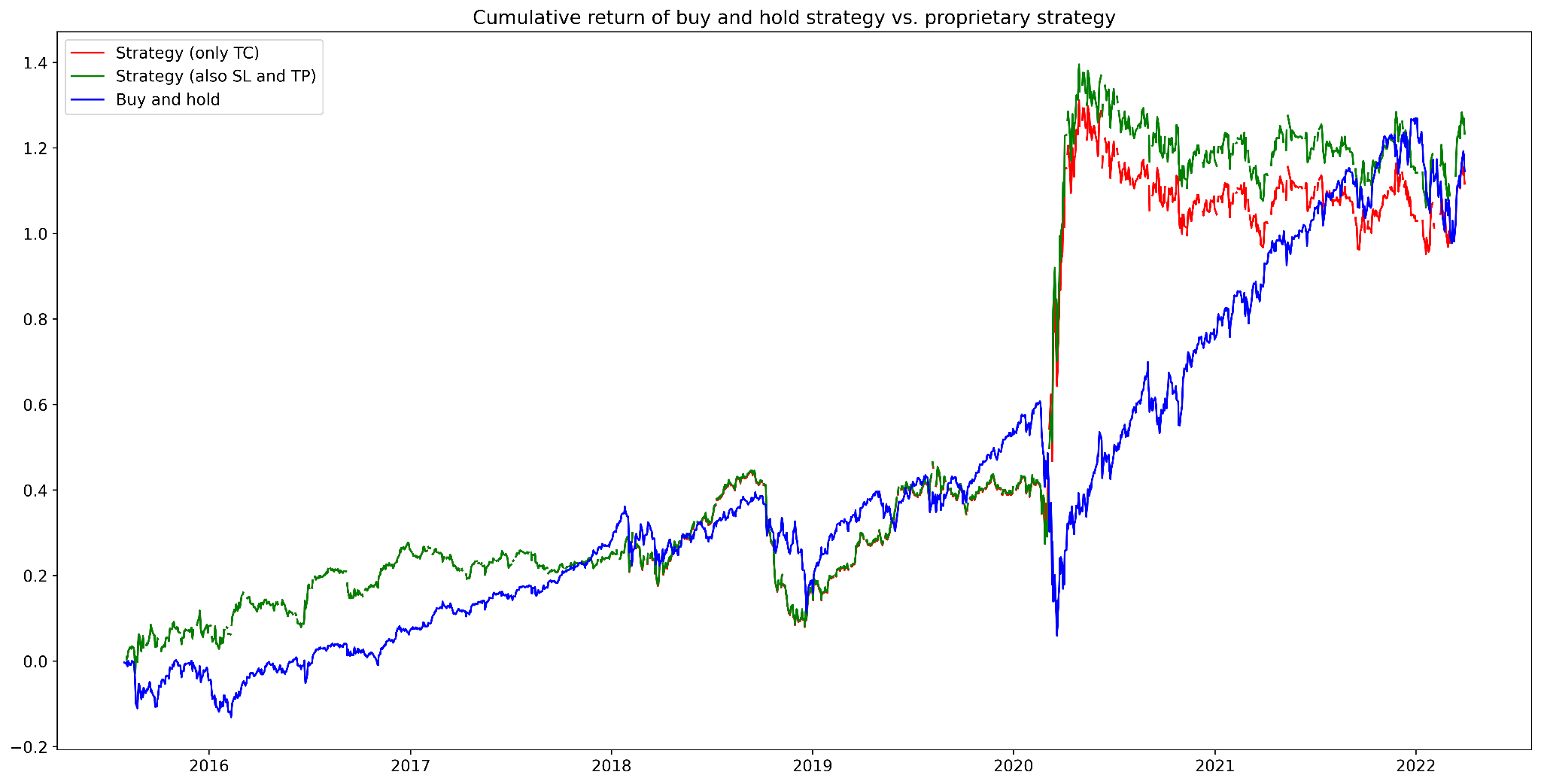
Figure 1. Cumulative returns of buy and hold strategy vs. proprietary strategy (daily data)

Source: Bocconi Students Investment Club

In the figure above, the green pattern depicts cumulative returns when a stop loss is set at 0.04. The buy and hold strategy and the proprietary one are strongly linearly correlated, with a Pearson coefficient of 0.85, and the proprietary strategy is moderately correlated with the VIX, with a Pearson coefficient of 0.46.

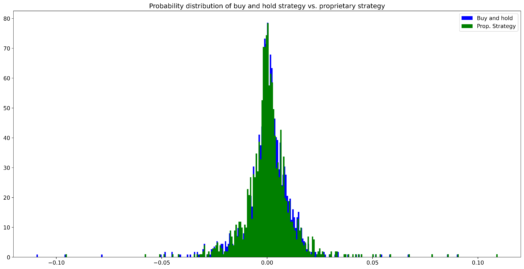
Figure 2. Probability distribution of buy and hold strategy vs. proprietary strategy (daily data)

Source: Bocconi Students Investment Club

The proprietary strategy exhibits a slightly higher mean and significantly higher skewness:

	Proprietary strategy	Buy and hold
Mean
Skewness
6-years Sharpe ratio

Figure 3. Key results of buy and hold strategy vs. proprietary strategy (daily data)

Source: Bocconi Students Investment Club

Bibliography

Kelly B.T. et al; (Re-)Imag(in)ing Price Trends; 2020

Basak S. et al; Predicting the direction of stock market prices using tree-based classifiers; 2018

Khanal A. et al; Stock price reactions to stock dividend announcements: A case from a sluggish economic period; 2017

Day Y., Zhang Y.; Machine Learning in Stock Price Trend Forecasting; 2013

Nikfarjam A. et al; Text mining approaches for stock market prediction; 2010

Basaka S. et al; Predicting the direction of stock market prices using tree-based classifiers; North American Journal of Economics and Finance; 2018

Ariyo A. A. et al; Stock Price Prediction Using the ARIMA Model; 2014