Introduction
This article is the first in Trading the Network, a seven-part series investigating whether relationships across financial assets contain predictive information that can ultimately be converted into tradable signals. Part I establishes the baseline by asking whether a simple network of historical return correlations improves equity return prediction at all. The subsequent articles progressively move from statistical similarity toward predictive information transmission: examining how financial edges should be defined, whether lead-lag and residual relationships improve the network, how shocks propagate across connected assets, when network effects become economically relevant, whether apparent improvements survive falsification and robustness tests, and finally whether any surviving predictive information remains profitable after portfolio construction and trading costs. The series therefore develops from the deliberately simple question: does adding a graph help? This leads toward identifying what a genuinely predictive and tradable financial network should look like.
Financial markets are naturally interconnected, yet many predictive models treat securities as independent observations. Graph Neural Networks (GNNs) offer an alternative because they allow information to propagate across relationships between assets. This article develops that idea from first principles and tests it in a deliberately transparent equity-selection experiment. A dynamic graph of large-cap US equities is constructed from trailing return correlations, and four forecasting models of increasing complexity are compared: Ridge regression, a conventional multilayer perceptron (MLP), a Graph Convolutional Network (GCN), and a Graph Attention Network (GAT). All models use the same stock-level inputs and forecast five-day cross-sectional return ranks. Their predictions are converted into the same weekly long-short strategy, and a random-graph GAT provides a falsification test for whether any apparent graph advantage comes from genuine network structure.
From Artificial Intelligence to Machine Learning
Suppose that for stock i at time t we observe a collection of characteristics,

and wish to predict some future quantity  . A machine-learning model seeks a function
  such that

where  denotes the model’s prediction and
  denotes the quantity that is subsequently realised. Supervised learning simply means that historical examples contain both sides of this relationship: the model observes earlier values of
  together with the later outcome , and attempts to learn a mapping that generalises to observations that were not used during training.
In this experiment, the inputs contain seven economically intuitive characteristics: the previous one-day, five-day, twenty-day and sixty-day returns, twenty-day realised volatility, twenty-day average dollar trading volume and sixty-day market beta. Symbolically,

These variables contain different forms of information. Recent returns capture short- and medium-horizon momentum or reversal. Realised volatility describes the magnitude of recent price fluctuations. Dollar volume provides information about liquidity and trading activity. Beta measures the sensitivity of an individual security to movements in the broader market. Before estimation, the features are standardised cross-sectionally. A characteristic  is transformed as
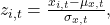
where  and
and  are respectively the cross-sectional mean and standard deviation of the characteristic at date t. A value of z = 2, for example, indicates that the stock lies two standard deviations above the contemporary cross-sectional mean. This transformation matters because the model is solving a relative forecasting problem. A 2% weekly return means something different when the rest of the market has fallen by 5% than when comparable securities have risen by 10%. Cross-sectional standardisation encourages the model to interpret a security relative to the opportunity set that existed at that moment.
What are we trying to predict?
Rather than forecasting exact returns, our strategy focuses on relative performance. Suppose stock A subsequently returns 4% and stock B returns 2%. A model predicting 8% for A and 6% for B is inaccurate about the magnitude of both returns, but it has still made the economically useful prediction that A will outperform B. For a strategy that buys predicted winners and shorts predicted losers, getting this relative ordering correct is more important than forecasting the exact percentage return.
We first calculate each stock’s subsequent five-day return. In simplified notation,
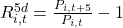
where Pᵢ,ₜ is the stock’s starting price and Pᵢ,ₜ₊₅ is its price five trading days later. In the actual backtest, information is observed after the market closes on date t, and positions can only be entered at the next available opening price. This prevents look-ahead bias, which would occur if the model were allowed to use information from today’s close while also pretending that it could already have traded at that same closing price.
Rather than asking the model to predict the exact five-day return, we rank all stocks according to their future returns. Suppose five stocks subsequently return −4%, −1%, 1%, 3%, and 6%. The stock returning 6% is ranked as the strongest performer, while the stock returning −4% is ranked as the weakest. These positions are then converted into percentile ranks. A stock at the 90th percentile performed better than approximately 90% of the other stocks, a stock around the 50th percentile was near the middle of the group, and a stock around the 10th percentile was among the weakest performers.
For convenience, we transform this percentile ranking from approximately zero to one into a scale running from −1 to +1:

where Fₜ(R⁵ᵈᵢ,ₜ) represents the stock’s percentile position within the cross-section. For example, a stock at the 90th percentile receives

a stock at the 50th percentile receives 0, while a stock at the 10th percentile receives −0.80. Values approaching +1 therefore represent future winners, values around zero represent stocks near the middle of the cross-section, and values approaching −1 represent future losers.
The forecasting process can therefore be summarised as current information → predicted score → predicted ranking → future realised ranking. The model succeeds when stocks that it ranks highly subsequently tend to outperform stocks that it ranks poorly. This is why we focus on the rank Information Coefficient (IC), which measures how closely the model’s predicted ordering corresponds to the ordering that occurs:

A positive IC means that stocks receiving higher predicted scores tended to achieve higher subsequent returns. An IC close to zero means that the predicted ranking contained little information, while a negative IC means that the model tended to rank future losers above future winners.
The Simplest Benchmark: Ridge Regression
Before introducing neural networks, we require a model capable of establishing how much information exists in the features without complex nonlinear processing. A conventional linear model assumes

Each coefficient measures how the prediction changes when the corresponding characteristic changes, holding the remaining characteristics constant. The difficulty is that financial characteristics are often correlated. One-day, five-day and twenty-day momentum, for example, are not independent measurements. Unrestricted estimation can consequently produce unstable coefficients that react strongly to noise in the training sample. Ridge regression addresses this through regularisation. Instead of minimising only squared prediction error,

it minimises

The first term measures the model’s prediction errors, so minimising it encourages the model to fit the historical data accurately. The second term, ∑ⱼβⱼ², measures the overall size of the model’s coefficients. Adding this term makes large coefficients costly, encouraging Ridge to keep them closer to zero unless the data provide sufficiently strong evidence that a large coefficient genuinely improves prediction.
The parameter λ determines how strongly this penalty matters. If λ = 0, there is no penalty and Ridge reduces to ordinary linear regression. As λ becomes larger, large coefficients are punished more heavily and the model becomes increasingly conservative. In our implementation, λ = 10, meaning that the model deliberately sacrifices some ability to fit the training data in exchange for more stable coefficients and, hopefully, better predictions on unseen data.
This creates a bias–variance trade-off. Bias refers to systematic error created when a model is too restricted to reproduce the true relationship in the data. Ridge deliberately introduces some additional bias by shrinking its coefficients towards zero: even when a characteristic genuinely matters, its estimated effect is pulled towards a more conservative value. Variance refers instead to how much the fitted model would change if it were trained on a slightly different sample. A highly flexible or unstable model may fit one historical sample extremely well but estimate very different coefficients when only a small number of observations change. Such a model has high variance and is more likely to have learned noise rather than a relationship that will persist.
Neural Networks: Learning Nonlinear Functions
Instead of mapping the original features directly into a prediction, a neural network passes them through intermediate computational units called neurons. These neurons learn combinations of the original variables, transform those combinations nonlinearly, and pass the resulting information to subsequent layers. The purpose is to allow the model to discover relationships that cannot easily be represented by a single straight-line equation. Consider one artificial neuron. Suppose its inputs include momentum, volatility and beta. The neuron first calculates a weighted combination of those variables,

Here x is the vector containing the input variables, while w contains a separate weight for each input. A weight determines how strongly that variable influences the neuron. A large positive weight means that higher values of the variable push z upwards, while a negative weight pushes it downwards. The term b, called the bias, is an intercept that allows the neuron to shift its output rather than forcing the relationship to pass through zero. The notation wᵀx simply represents multiplying each input by its corresponding weight and adding the results together. For example, imagine that a neuron receives only momentum and volatility. It might eventually learn something resembling

The numbers 0.8, −0.3 and 0.1 are not specified by the researcher. They are learned from the training data. In this example, stronger momentum increases the neuron’s intermediate value, while higher volatility reduces it. If the model stopped here, however, the neuron would still be performing a linear calculation. Neural networks become substantially more powerful because the weighted sum is passed through an activation function:

The function ϕ introduces nonlinearity. Without it, stacking many neural-network layers would ultimately remain equivalent to another linear transformation. The activation function allows the effect of one variable to depend on the state of other variables and allows the network to represent curved, threshold-like and interacting relationships. A single neuron can only learn one such transformation, so neural networks combine many neurons into layers. The first hidden layer can be written as

These learned variables are called hidden representations because they are created internally by the network rather than directly observed in the dataset. One neuron might become particularly sensitive to strong short-term momentum combined with low volatility, while another might react to high beta and unusual trading activity. We do not manually define these combinations. The network determines which combinations are useful for reducing prediction error. A second layer then takes the first layer’s learned representation as its input:

This allows the model to combine already-learned patterns into more complicated patterns. The final layer converts this internal representation into the prediction:

The complete process can therefore be understood as original features → hidden layer 1 → hidden layer 2 → prediction. Our model is a Multilayer Perceptron, or MLP, with hidden representations of dimension 32.
The next question is how the network discovers appropriate values for potentially thousands of weights and biases. This process is called training. At the beginning the network makes predictions, compares those predictions with the historically observed targets, measures how wrong it was using a loss function, and then adjusts its parameters in an attempt to reduce that error.
If θ represents all parameters in the neural network, training seeks

The notation arg min simply means: find the parameter values that make the loss as small as possible. The loss is a numerical measure of prediction error. A smaller loss indicates that the network’s predictions are closer to the targets in the training data.
The network learns through gradient-based optimisation. The gradient, ∇θ(θ), measures how the loss would change if each parameter were moved slightly. It therefore tells the optimisation algorithm which direction would increase the error and, consequently, which opposite direction should reduce it. Parameters are repeatedly updated according to

Here k denotes the current optimisation step and η is the learning rate. The learning rate controls how large each adjustment is. If it is too large, the optimiser may repeatedly jump past good parameter values and training can become unstable. If it is too small, learning can become extremely slow. Our implementation uses η = 0.001.
One complete pass through the training dataset is called an epoch. The model is allowed to train for a maximum of 120 epochs. This does not mean that it necessarily uses all 120. Continuing to minimise training error indefinitely creates the danger of overfitting. A sufficiently flexible neural network may begin learning peculiarities and random noise belonging specifically to the training sample rather than relationships that generalise to unseen observations.
To reduce this risk, the model uses several forms of regularisation. The first is weight decay, set to 0.0001. Weight decay operates similarly in spirit to the Ridge penalty discussed previously: it discourages the network from relying on unnecessarily large parameter values. This encourages a smoother and less extreme fitted model.
The second technique is dropout, set to 10%. During training, dropout randomly switches off approximately 10% of the relevant hidden activations on each pass. The network therefore cannot rely excessively on one neuron always being present. It is encouraged to distribute useful information across several parts of the network. An intuitive analogy is repeatedly forcing a team to operate with a few randomly absent members; the team becomes less dependent on any single individual.
The third safeguard is early stopping. The data used for model development are divided into training and validation periods. Parameters are learned using the training sample, while performance is repeatedly checked on the separate validation sample. If training performance continues improving but validation performance stops improving, this is evidence that the model may be beginning to memorise the training data rather than learning relationships that generalise.
Our early-stopping patience is fifteen epochs. This means that training is terminated if validation performance fails to improve for fifteen consecutive epochs. The model then retains the parameter state associated with the strongest validation performance rather than automatically using the final training epoch.
From Independent Stocks to a Graph
An MLP still treats every stock as an independent observation. A GNN changes the structure of the problem. Before introducing the matrices, it helps to picture what a graph actually is. A graph is simply a collection of objects and the relationships connecting them. The objects are called nodes and the relationships are called edges. In this article, every node is a stock. If Nvidia is connected to AMD, Broadcom and TSMC, the four companies are nodes and the lines linking Nvidia to the other three are edges. The graph therefore turns the stock universe from a table of independent rows into a network in which selected stocks are allowed to interact.
This distinction matters because the graph and the neural network are separate objects. We construct the graph first from historical market data; the graph determines which stocks are connected. The GNN is then placed on top of that graph and determines how information is exchanged across those connections. A poor result can therefore arise because the graph identifies the wrong relationships, because the neural architecture processes those relationships badly, or because both problems occur at the same time.

where  is a collection of nodes and
  a collection of edges. In our financial graph,

An edge between stocks  and
and  indicates that the two securities are statistically related according to their recent returns. This relationship can be represented by an adjacency matrix,
The adjacency matrix is simply the numerical version of this network map. To make this concrete, imagine a four-stock graph containing Nvidia, AMD, Broadcom and TSMC in which Nvidia is connected to each of the other three, while those three are not directly connected to one another. If we order the rows and columns as NVDA, AMD, AVGO and TSM, the adjacency matrix is
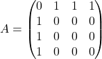
Each row and column refers to one stock. A value of 1 means that the corresponding pair is connected, while a value of 0 means that no edge exists between them. The zeros on the diagonal mean that we have not yet added self-connections. The matrix itself is simply a form that a computer can use to store the network and decide which nodes may exchange messages.
The critical modelling question is therefore how an edge should be defined. We estimate the trailing sixty-day return correlation

The phrase top-k neighbours simply means that we keep only the k strongest relationships for each stock. For example, suppose Nvidia’s sixty-day correlations with AMD, Broadcom, TSMC and JPMorgan were 0.82, 0.76, 0.71 and 0.08. If k were equal to 2, Nvidia would keep AMD and Broadcom as its two neighbours because they have the two highest positive correlations. TSMC and JPMorgan would remain in the investment universe but would not be directly connected to Nvidia in that particular graph.
For each security, the baseline graph retains its ten most positively correlated neighbours. The graph is symmetrised, so if one security selects another as a neighbour the relationship becomes available in both directions. Self-connections are subsequently introduced inside the graph convolution so that a stock’s own representation is not discarded. The graph is dynamic. A relationship observed in 2018 need not remain identical in 2022. Each date uses only the historical return information available at that point.
Graph Neural Networks and Message Passing
The defining operation of a GNN is message passing. Four terms are useful here. A feature is an observed input such as momentum or volatility. A representation, sometimes called an embedding, is the collection of learned numbers used internally by the neural network to describe a stock after those raw features have been transformed. A message is the information one node sends to another through an edge. Message passing is the repeated process of collecting those messages and using them to update each stock’s representation.
The simplest way to remember the division of labour is that the graph determines who is allowed to communicate, while the GNN determines how that communication changes the representation of each stock. The graph therefore supplies the communication channels; message passing supplies the computational rule operating through those channels.

A graph layer allows the stock to receive information from its neighbours,

A simplified update is

In layman’s terms, the model combines what it already knows about stock i with information received from connected stocks and constructs a new representation. The process can be repeated. After one graph layer, a stock incorporates information from its direct neighbours. After two layers, information can indirectly arrive from neighbours of those neighbours.
Graph Convolutional Networks
A Graph Convolutional Network (GCN) is a neural network designed for data in which observations are connected. In this study, each node is a stock and each edge links two stocks that the graph treats as related. The word convolution sounds more complicated than the idea itself. In an image, a convolution combines information from nearby pixels. In a graph, there is no fixed left, right, up or down, so the relevant neighbourhood is defined by the edges. A graph convolution therefore means combining information from a node with information from its graph neighbours.
A GCN needs to preserve each stock’s own characteristics. It therefore adds a self-connection to every node by adding the identity matrix  :
:

The identity matrix contains ones on its diagonal and zeros elsewhere, so this operation connects every stock to itself. Nvidia can therefore receive information from AMD, Broadcom and TSMC without discarding Nvidia’s own representation.
Different stocks can have different numbers of neighbours. If one stock has three connections and another has twenty, simply adding all incoming information would mechanically give the more connected stock a larger message. The GCN therefore uses the degree matrix  , which records how many connections each node has, to normalise the graph. The normalised adjacency matrix is

After this normalisation, the complete GCN layer can be written as

Here  contains the current representations of all stocks at layer
  . At the start,
  , so the representations are simply the observed stock features. The normalised adjacency matrix determines who exchanges information and how strongly the graph scales that exchange. Multiplication by collects neighbour information,
  contains trainable neural-network weights that transform it, and
  is the nonlinear activation function.
For Nvidia, a simplified version is

where the  terms represent graph-normalisation weights. The important point is that Nvidia’s new representation is now a mixture of its own state and information from its neighbours. This process is called message passing.
The potential benefit is that related stocks may contain useful shared information. The risk is smoothing: repeatedly mixing neighbouring representations makes connected stocks more similar. If two nodes initially have values of 1 and 5, averaging them moves both toward 3 and reduces their difference. This can help when common information is signal and stock-specific variation is noise, but it can hurt a cross-sectional strategy if the difference between two connected stocks is exactly what predicts which one will outperform. A GCN therefore makes a strong assumption: neighbour information is useful to combine rather than useful because it differs.
Graph Attention Networks
A Graph Attention Network (GAT) keeps the same basic message-passing idea as a GCN but addresses one important limitation: different neighbours should not necessarily matter equally. The simplest distinction is that a GCN asks which stocks are my neighbours?, while a GAT additionally asks which of those neighbours should I listen to most? The candidate graph can therefore be identical in both models. What changes is how strongly each permitted neighbour influences the stock being updated.
Suppose stock is being updated and stock is one of its neighbours. Their current representations are  and
and  . These representations contain the information currently held by the network about each stock: in the first layer this ultimately comes from observed features such as momentum, volatility, liquidity and beta, while in later layers it may already contain learned combinations of those features. The GAT first applies a learned transformation
  and then compares the transformed representations through a learned scoring function:

The resulting  is a raw attention score. It answers a very specific question: given the current representations of stocks and , how relevant does neighbour appear when constructing the next representation of stock ? If is Nvidia and is AMD, then
  is the model’s current relevance score for AMD when updating Nvidia. Importantly, this is not a permanent importance score attached to AMD. The score is produced by a learned function of the stocks’ current representations, so the same neighbour can receive different importance in different market states.
Nothing tells the model in advance that AMD should matter more than TSMC. The attention rule is learned from the forecasting task itself. At the beginning of training, the parameters inside and  do not yet encode a useful rule. The GAT makes return-rank predictions using its current parameters, compares those predictions with the historical targets, and calculates a loss
  measuring prediction error. Backpropagation then asks how sensitive that loss is to every trainable parameter
  in the network:

Gradient descent updates the parameter in the direction expected to reduce the loss:

where  is the learning rate. A parameter with a larger gradient is changed more at that optimisation step because the loss is more sensitive to it; a parameter with a small gradient changes less. The model is therefore not directly told to increase or decrease AMD’s weight. Instead, backpropagation changes the shared parameters that generate attention scores. If parameter changes that make AMD relatively more influential repeatedly reduce forecasting error in situations resembling the current one, the learned scoring rule will tend to assign AMD a larger score in similar situations in the future.
This explains how one neighbour receives more attention than another. For a given target stock, the same learned scoring rule is applied to each eligible neighbour. Suppose Nvidia’s current raw scores are  ,
,  and
and  . AMD receives the largest raw score because, under the parameters learned from past prediction errors, the current Nvidia-AMD representations look more relevant to the forecasting task than the other pairs. These raw scores are then converted into positive, comparable weights using the softmax function:

For each target stock , the attention weights satisfy

The softmax therefore turns relative relevance scores into relative shares of attention. If Nvidia ultimately assigns weights of  to AMD,
  to Broadcom and
  to TSMC, AMD contributes more than three times as much as TSMC to that particular neighbourhood update.
Readers familiar with Transformer models may know attention through queries, keys and values. The GAT formulation used here does not explicitly create separate  ,
,  and matrices, so the analogy should not be taken literally. Conceptually, however, stock acts like a query: it is the node asking which neighbour is relevant. Neighbour provides information analogous to a key, because its representation helps determine whether it is relevant to . The transformed neighbour representation
  plays the role of the value: it is the information that is actually transferred if neighbour receives a high attention weight. In our GAT these roles are embedded inside the graph-attention scoring mechanism rather than written as the separate projections commonly used in Transformers.
Once the attention weights have been calculated, stock is updated according to

The equation can be read from the inside out. Each neighbour’s representation is transformed by , multiplied by its learned attention weight, and added to the other weighted neighbour messages. The activation function then applies a nonlinear transformation. In the Nvidia example, a simplified update could look like

Our actual experiment uses two attention heads. Both heads observe the same graph and underlying stock information, but each has its own attention parameters. They can therefore learn different ways of judging neighbour relevance. For the same Nvidia neighbourhood, one head could place relatively more weight on AMD while the other places more weight on Broadcom. Any such specialisation emerges from training; it is not imposed by the researcher. The two head outputs are then combined inside the same GAT before the final prediction is produced. They should therefore be understood as two parallel learned views of the same local network, not as two separate trading strategies.
Attention makes the GAT more flexible than a GCN, but it does not eliminate the basic aggregation problem. A GAT can learn how much to listen to AMD, yet it still mixes AMD’s information into Nvidia’s representation. If the useful trading signal lies in the difference between Nvidia and AMD rather than in their combined state, attention may still weaken that distinction. Greater flexibility therefore does not automatically imply better forecasting.
The four models can now be separated cleanly. Ridge uses only each stock’s own features in a regularised linear model. The MLP still uses only the stock’s own features but allows nonlinear relationships. The GCN adds information from graph neighbours through normalised message passing. The GAT retains message passing but additionally learns which neighbour messages deserve more or less weight. The empirical hierarchy is therefore

Each step adds a specific form of modelling flexibility. The relevant question is not which model is most sophisticated, but whether each additional layer of complexity produces better out-of-sample forecasts.
Experimental Design and Backtest Construction
The development universe consists of current S&P 500 constituents with historical market data beginning in 2010. Securities are subject to minimum history, price and liquidity conditions, including a minimum price of  and average dollar volume of
  . This design creates a useful large-cap cross-section, but it contains an important limitation: using today’s index members historically creates survivorship bias. Firms that left the index or disappeared entirely are not represented symmetrically with surviving firms. The present experiment should therefore be interpreted primarily as a controlled comparison of model architectures rather than a final publication-quality estimate of historical implementable returns. A point-in-time constituent universe is required in the next research stage.
The reported Ridge, MLP, GCN and GAT specifications are fixed representative implementations, not an exhaustive search over every possible architecture and hyperparameter combination. The evidence therefore speaks to these tested implementations and to this correlation-graph design; it should not be interpreted as a general rejection of the GNN model class.
Signals are formed weekly. The model forecasts five-day cross-sectional performance and the portfolio buys the highest-ranked 10% of securities while shorting the lowest-ranked 10%. If  and
and  denote the long and short sets,
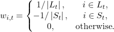
This produces approximately zero net exposure,

while maintaining positive gross exposure on both sides. The strategy is intentionally simple. If sophisticated portfolio optimisation were introduced simultaneously with the GNN, improvements could not confidently be attributed to the forecasting architecture.
Transaction costs are incorporated through turnover. Let

Net portfolio return is then

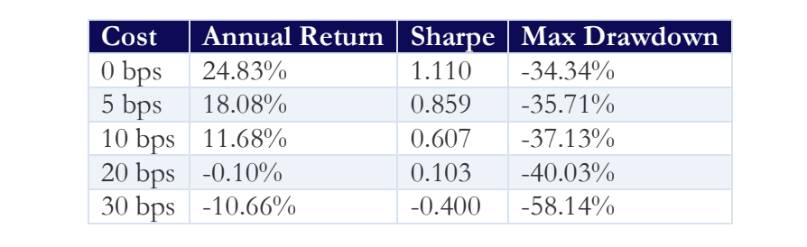
where  is the assumed cost per unit of turnover. The baseline result uses ten basis points, and additional results are reported at zero, five, twenty and thirty basis points.
Machine-learning datasets are therefore commonly divided into three different parts: training data, validation data and test data. Each has a different purpose. The training sample is the data from which the model actually learns its parameters. For Ridge regression, this means estimating the coefficients beta. For a neural network, it means repeatedly adjusting the weights and biases in order to reduce the training loss. The model is therefore allowed to see the training observations many times.
The validation sample is different. It is used to make decisions about the modelling process itself. For example, a neural network may continue improving its fit to the training data even after it has begun to overfit. We therefore evaluate its performance on the separate validation period after each training epoch. If training performance continues improving while validation performance stops improving, this suggests that the model is learning details specific to the training sample rather than relationships that generalise to unseen data. Our early-stopping procedure uses this validation performance to decide when training should stop.


Since validation data influence decisions such as when training stops, they are no longer completely untouched. The test sample is the final unseen period. In many conventional machine-learning applications, observations are randomly divided between these three samples. This is inappropriate for our financial problem because time has a natural direction. We therefore use chronological walk-forward testing. The first out-of-sample test year is 2018 and the final test year is 2025. For each stage of the experiment, earlier observations form the training sample, the most recent historical period is used for validation, and the subsequent period is reserved for testing.
Measuring Predictive Information
Since the objective is ranking, the primary measure is Spearman rank correlation,

If  , higher model scores tend to correspond to higher subsequent returns. If
  , there is no systematic ranking relationship. If
  , the ordering tends to be wrong.
Financial ICs are usually small because future individual-stock returns contain enormous idiosyncratic noise. What matters is whether a small positive relationship persists across many securities and dates. We therefore also report the IC information ratio,
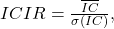
which measures average predictive correlation relative to its variation through time. Pearson IC is reported as a secondary diagnostic, but rank IC is the natural primary statistic for a rank-based portfolio.
Baseline Forecasting Results
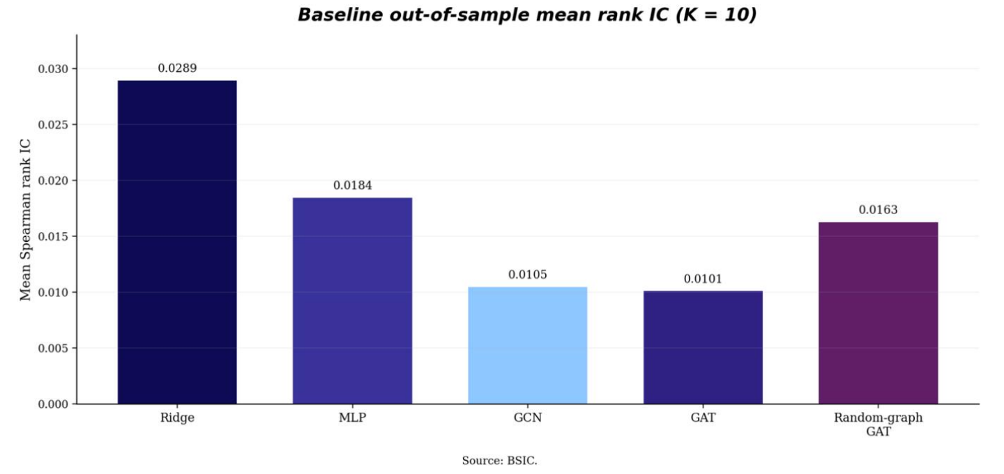
At the baseline graph density of ten neighbours, Ridge regression produces the highest mean rank IC, equal to  . The MLP falls to
  . The GCN produces
  , while the GAT produces
  . The random-graph GAT produces
  . The corresponding IC information ratios are
  for Ridge,
  for the MLP,
  for the GCN,
  for the GAT and
  for the random-graph GAT.
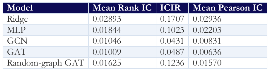
The point estimates reveal two distinct deteriorations in predictive information. First, Ridge outperforms the MLP, indicating that additional nonlinear flexibility does not improve this feature set in the present experiment. Second, the MLP outperforms both GCN and GAT, indicating that neighbourhood message passing is associated with a further decline in predictive quality. This distinction prevents us from simply concluding that “neural networks fail”. The evidence is narrower: the tested nonlinear model does not improve on Ridge, and the tested correlation-based graph architectures perform worse still.
Portfolio Results
At ten basis points of assumed transaction cost, Ridge produces an annualised return of  , annualised volatility of
  , a Sharpe ratio of
  , and a maximum drawdown of
  . Average turnover is
  under the implemented convention, and the weekly hit rate is
  .
.
The MLP remains positive but substantially weaker, producing an annualised return of  and Sharpe ratio of
  . Its maximum drawdown is
  . The GCN loses approximately per annum after costs and produces a slightly negative Sharpe ratio. The GAT performs worse still, losing approximately
  per annum, with a Sharpe ratio of
  and a maximum drawdown of
  . The random-graph GAT also loses money after costs.
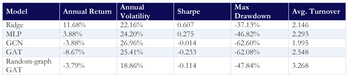 The ranking of trading performance therefore broadly agrees with the forecasting evidence. This agreement matters. If the GAT had possessed a superior IC but an inferior portfolio Sharpe, one might primarily suspect turnover or portfolio construction. Instead, the graph models already contain weaker predictive information before transaction costs are considered.
The Decile Test: Does the Model Order Returns Correctly?
One of the strongest pieces of evidence supporting Ridge comes from sorting securities into ten groups according to predicted score. For Ridge, the mean subsequent five-day return rises from approximately  in the lowest predicted decile to
  in the highest. The middle of the distribution is not perfectly monotonic, but the upper half shows a clear progression: deciles five through ten produce approximately
  ,
,  ,
,  ,
,  ,
,  and respectively.
The spread between the extreme groups is therefore approximately

over the five-day horizon. The relevant interpretation is that securities receiving higher Ridge scores tend, on average, to realise higher subsequent returns. This is exactly what a cross-sectional ranking model is intended to accomplish.
A decile analysis is important because a top-minus-bottom strategy can occasionally appear profitable due to a small number of extreme observations. A smoother relationship between predicted score and realised return provides stronger evidence of genuine ranking information. Ridge passes this test more convincingly than the GAT, whose decile structure is substantially less orderly.
Transaction Costs
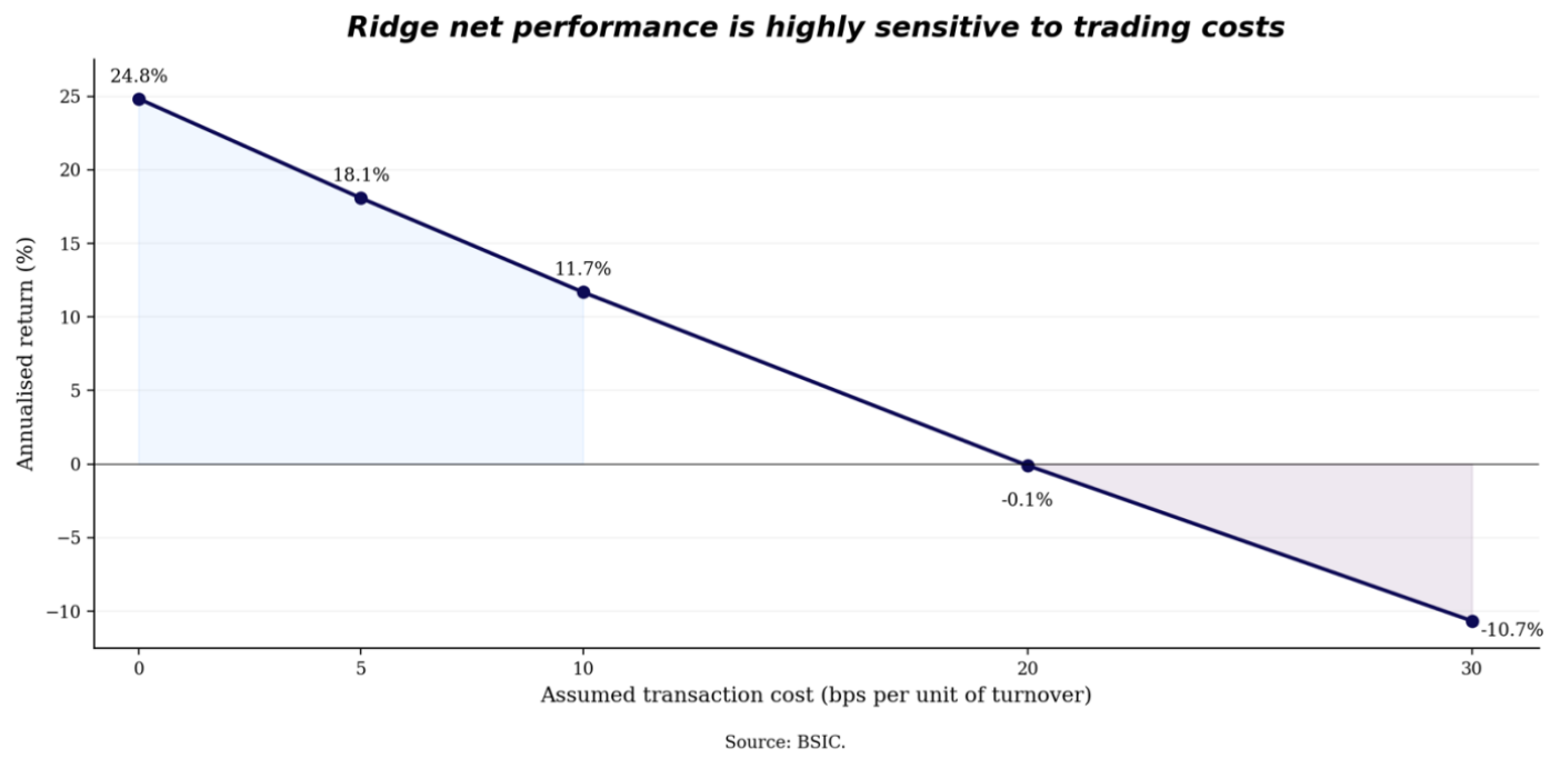
The Ridge strategy appears considerably stronger before transaction costs. At zero assumed cost, annualised return is  and Sharpe ratio is
  . At five basis points, annualised return falls to
  and Sharpe to
  . At ten basis points, the figures are and
  . At twenty basis points, annualised return is approximately zero and Sharpe falls to
  . At thirty basis points, annualised return becomes
  and Sharpe becomes negative.
The reason is turnover. Average Ridge turnover is approximately  per rebalance under the backtest convention. The strategy is therefore not simply forecasting returns; it is repeatedly paying to replace positions. The result exposes a fundamental distinction between statistical alpha and tradable alpha. A model can correctly identify small differences in expected return while still being economically unattractive if exploiting those differences requires excessive trading.
The GAT suffers from both problems simultaneously. Its underlying forecasting signal is weaker, and its average turnover is higher, at approximately  in the baseline specification. Transaction costs therefore magnify a problem that already exists at the prediction stage rather than creating the problem from scratch.
Performance Through Time
Ridge’s net annual returns are positive in 2018, 2019, 2020, 2021, 2022, 2023 and 2024. The corresponding returns are approximately  ,
,  ,
,  ,
,  ,
,  ,
,  and
and  . Performance turns negative in 2025, at approximately
  .
.
The strongest annual Sharpe ratios occur in 2019 and 2022, at approximately 1.04 and 1.10 respectively. The unusually high absolute return in 2020 occurs alongside much greater volatility, which keeps the Sharpe below one. The distribution across calendar years is consistent with the signal not being generated by a single profitable episode, although the experiment does not formally classify or test market regimes. The deterioration in 2025 nevertheless warns against interpreting the relationship as permanent.
The GAT tells a very different story. Its net return is negative in seven of the eight test years. Only 2020 is positive, producing approximately  . Returns are materially negative in 2022 and 2023, at approximately
  and
and  respectively. The graph model therefore does not merely experience one unfortunate regime. Under this specification, its weakness is persistent.
Does Graph Density Explain the Failure?
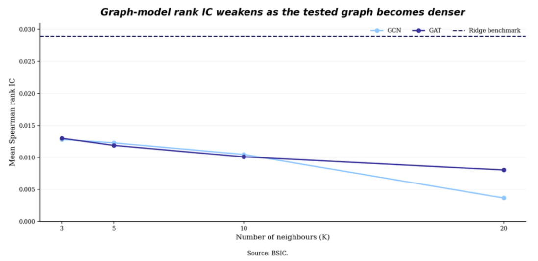
Perhaps ten neighbours is simply the wrong network density. To investigate this possibility, the complete experiment was repeated using

The conclusion survives. GCN rank IC changes from approximately  at
at  to
to  at
at  , at
, at  , and only
  at
at  . The progression is therefore

GAT follows a similar pattern:

Across the tested values of K, increasing graph density is associated with deteriorating predictive power, a pattern consistent with an information-dilution hypothesis. As additional neighbours are introduced, each security’s representation contains more common information and less purely stock-specific variation. This sensitivity exercise does not establish that denser graphs causally reduce forecasting power, but it is consistent with the mechanism that conventional message passing becomes less aligned with a cross-sectional ranking objective as neighbourhood aggregation broadens.
Ridge, by construction, is unchanged across these graph-density experiments. Its mean rank IC remains and its ten-basis-point Sharpe remains . This stability provides a useful reference because the observed deterioration is specific to the graph architectures rather than a change in the underlying test sample.
Why Might the GNN Fail? Correlation Is Not Predictive Direction
The first potential problem lies in the graph itself. We connect securities because

has recently been high. Correlation tells us that two securities have moved together. It does not tell us that one contains information useful for forecasting the other.
Consider two stocks driven simultaneously by the market. The true economic structure may be

and

Then  even though neither security leads the other. A correlation graph nevertheless represents the relationship as

The edge therefore reflects shared exposure rather than information transmission. Message passing subsequently treats the two observations as if exchanging their representations is likely to improve prediction. That is not implied by contemporaneous correlation.
This distinction may be the most important weakness. A graph built from similarity is not necessarily a graph of predictive influence. For a forecasting problem, what we would ideally like to identify is something closer to

where information in security  precedes and helps predict a later movement in security
  .
.
The Graph May Be Removing Exactly What We Want to Predict
Cross-sectional stock selection depends on differences between securities. Suppose two neighbouring securities possess representations  and
and  . Message passing constructs something resembling

If and are genuinely similar firms, their common component becomes stronger. Yet the strategy is not trying to predict their common component. It is trying to predict which one will outperform the other.
Suppose their representations can be decomposed as

and

where  is a common factor and
  contains stock-specific information. Graph averaging strengthens the shared component while potentially reducing the relative distinction contained in

Yet that relative distinction may be precisely where cross-sectional alpha resides. A correlation graph may therefore be excellent at learning what stocks have in common while our trading objective depends on learning how they differ.
Over-Smoothing and the Geometry of the Prediction Problem
The preceding intuition generalises into the mathematical phenomenon of over-smoothing. Repeated graph convolution can cause node representations to become increasingly similar. For connected securities and , deeper propagation can push the system towards

In a classification problem where connected nodes usually share the same class, this may be useful. In a cross-sectional ranking problem, it can be destructive. Our objective requires dispersion in predictions,

whereas smoothing pushes representations towards similarity,

The architecture and objective may therefore be partially opposed. The empirical relationship between increasing and declining GCN/GAT IC is consistent with this mechanism. It does not prove that over-smoothing is the unique cause, but it is exactly the pattern one would expect if additional neighbour aggregation progressively removes the cross-sectional differences that matter for ranking.
The Random-Graph Falsification Test
The random graph provides another useful falsification test, although its behaviour is not uniform across graph densities. At , random-graph GAT rank IC collapses to approximately  , far below the real GAT’s
  . This suggests that the real sparse network contains some structure.
At larger graph densities, however, the random graph becomes surprisingly competitive. At ,

compared with

At ,

compared with

This warns that a flexible graph architecture can create useful-looking representations for reasons that are not straightforwardly attributable to economically meaningful edges. Moreover, the random-graph portfolios remain economically poor after costs. At , the random GAT produces a negative annual return and negative Sharpe despite its higher IC than the real GAT.
This falsification is also consistent with a broader lesson from the financial-GNN literature: relation choice is itself part of the model. Published stock-prediction architectures have therefore experimented with sector/company links, learned dynamic relations, hypergraphs and sparsification rather than relying on one generic correlation network. Part I does not optimize across those alternatives; its purpose is to establish a transparent baseline that later articles can try to falsify and improve.
The Next Research Steps: From Correlation Networks to Predictive Networks
Subsequent research should begin from the failure identified above rather than attempting to optimize it away. The central research question should become: can a graph designed around information transmission rather than contemporaneous similarity make relational learning useful for cross-sectional equity prediction?
The first experiment will replace contemporaneous correlation with a directed lead-lag graph. Instead of measuring

we estimate relationships such as

or more generally

An edge would then have a predictive interpretation:  means that movements in historically precede movements in . Returns should also be residualised against broad common factors before relationships are estimated. For example,

A graph constructed from residuals  would be less likely to connect two securities merely because both possess high market or sector beta. The resulting edges would have a better chance of representing idiosyncratic information transmission rather than shared exposure. A second improvement should preserve the distinction between self-information and neighbour-information. Rather than immediately smoothing the two together, we can construct
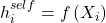
and separately

The final predictor can then learn

The difference term is particularly attractive because it directly represents whether the stock is behaving differently from its network. This may be far better aligned with cross-sectional alpha than conventional graph smoothing. The architecture would therefore shift from neighbour averaging towards a notion of neighbour pressure or relative dislocation.
Part II will also test edge sparsity much more aggressively. The Part I sensitivity exercise suggests that, within the tested range, adding neighbours is associated with weaker graph-model performance. A predictive graph may therefore benefit from testing only the strongest one, two, three or five directional relationships.
Conclusion
The original hypothesis was simple:

The empirical hierarchy is economically coherent but should remain narrowly interpreted. Ridge leads the baseline mean rank IC at 0.0289, the MLP falls to 0.0184, and the GCN and GAT fall to roughly 0.010. The portfolio evidence points in the same direction, but implementation is demanding: Ridge turnover is about 2.15 per rebalance and its annualised return falls from 24.83% before assumed costs to 11.68% at 10bp and approximately zero at 20bp. The current-constituent universe additionally introduces survivorship bias. The strongest result is the failure of added graph complexity to improve the same cross-sectional forecasting task under the tested design.
The experiment does not support that hypothesis in its simplest form. It also does not establish that GNNs are ineffective for equity prediction. What it shows is narrower: under a common feature set and chronological walk-forward design, the tested GCN and GAT architectures built on trailing contemporaneous-correlation graphs fail to improve on simpler stock-level benchmarks. Two companies can be economically related without displaying stable return correlation, and two stocks can be highly correlated without transmitting useful predictive information. The failure of the baseline therefore motivates the rest of the series: the question is not whether markets form networks, but whether the edges supplied to a forecasting model represent information that arrives early enough, persists long enough and survives implementation strongly enough to be tradable.
References
[1] Kipf, Thomas N.; Welling, Max, “Semi-Supervised Classification with Graph Convolutional Networks,” International Conference on Learning Representations (ICLR), 2017.
[2] Velickovic, Petar; Cucurull, Guillem; Casanova, Arantxa; Romero, Adriana; Lio, Pietro; Bengio, Yoshua, “Graph Attention Networks,” International Conference on Learning Representations (ICLR), 2018.
[3] Feng, Fuli; He, Xiangnan; Wang, Xiang; Luo, Cheng; Liu, Yiqun; Chua, Tat-Seng, “Temporal Relational Ranking for Stock Prediction,” arXiv:1809.09441, 2018.
[4] Cheng, Rui; Li, Qing, “Modeling the Momentum Spillover Effect for Stock Prediction via Attribute-Driven Graph Attention Networks,” Proceedings of the AAAI Conference on Artificial Intelligence 35(1), 2021, pp. 55-62.
[5] Uddin, Ajim; Tao, Xinyuan; Yu, Dantong, “Attention Based Dynamic Graph Neural Network for Asset Pricing,” Global Finance Journal 58, 2023, Article 100900.
[6] Gupta, Gautam; Goel, Priyanshi; Verma, Divyanshi; Malhotra, Amarjit, “SGAT-SP: Sparse Graph Attention Networks for Stock Prediction,” Journal of Forecasting, 2026.
[7] Standard & Poor’s Dow Jones Indices, “S&P 500,” index methodology and constituent information; used here only as background for the large-cap US equity universe. Historical point-in-time membership is not reconstructed in Part I.
[8] BSIC calculations and backtest outputs for Trading the Network I. All reported IC, portfolio, turnover, cost-sensitivity and graph-density results are generated by the study described in this article.


0 Comments