Beyond Traditional Lead-Lag Detection Methods

Download PDF

Introduction

Lead-lag relationships describe a simple claim: asset X may embed information about asset Y at two different points in time. If this delay is systematic and measurable than a model can exploit such a structure to produce forecasts and ultimately trading signals. The challenge is that the relevant dependency structure is typically sparse, delayed, and state-dependent: only a subset of assets carries predictive content for any given target, the informative lag may differ across pairs and across dates, and the strength or even sign of the relationship may shift across volatility, liquidity, or macro regimes. In advanced settings, lead–lag models are therefore not merely estimating correlations; they are attempting to infer a dynamic, non-linear transmission structure through which information propagates across markets and to translate that structure into forecasts, rankings, and ultimately trading signals.

To approach this problem this article explores two separate methods aimed at capturing non-linear lead-lag relationships and therefrom producing trading signals. The first is the Levy Area and the second is a system machine learning architecture first named DeltaLag in its proposed paper. 

Model I: The Lévy Area

Traditional lead–lag models have long relied on tools such as autocorrelation structures and Granger causality tests, but both models carry respective flaws. Autocorrelation-based methods are fundamentally limited by their insensitivity to the direction of time. The correlation structure remains unchanged under time reversal, making it difficult to distinguish genuine lead–lag effects from symmetric co-movement. Moreover, Granger causality typically relies on linear specifications, assuming that predictive relationships can be captured through linear combinations of past values. These limitations motivate the need for a more flexible framework: the Lévy area approach.

At its core, the Lévy area is a geometric quantity that measures how two time series evolve relative to each other over time. It is a crucial part of rough path theory, where higher-order integrals encode path structure beyond simple increments, and functions to capture second-order temporal structure unlike simple covariance. Intuitively, consider two continuous paths and If you plot on a plane as time evolves, you trace out a curve. The Lévy area measures the signed area enclosed by this curve and the straight line connecting its endpoints. If the path loops counterclockwise, the area is positive; clockwise gives negative area. This immediately hints at directionality which gives a key idea for lead–lag detection. 

For sufficiently smooth paths, the Lévy area over an interval is:

were

• shows how Y moves when X is “large”
• shows how X moves when Y is “large”

The difference between the two captures asymmetry in their interaction over time. If the two processes move simultaneously with no structure, the Lévy area tends to average out. But if one tends to move before the other, a consistent signed area emerges.

This makes the Lévy area particularly valuable for prediction in mathematical finance. Rather than imposing a fixed lag or relying on parametric models, it offers a model-free, path-wise approach to uncovering causality-like effects embedded in the data. This is especially relevant in modern markets where information propagates continuously and at varying speeds across instruments.

Lead-lag in commodity markets 

Commodity markets are a natural setting for such analysis because they exhibit structural lead–lag relationships driven by physical and economic constraints. A central example is the crack spread, which captures the pricing relationship between crude oil and its refined products such as gasoline or diesel, where upstream inputs typically lead downstream outputs due to the production chain. A similar concept appears in agricultural markets through the crush spread, which links inputs like soybeans to outputs such as soybean oil and meal. More broadly, commodities also display horizontal relationships across closely linked markets, such as gold and silver, where shared demand drivers and substitution effects create interconnected price dynamics.

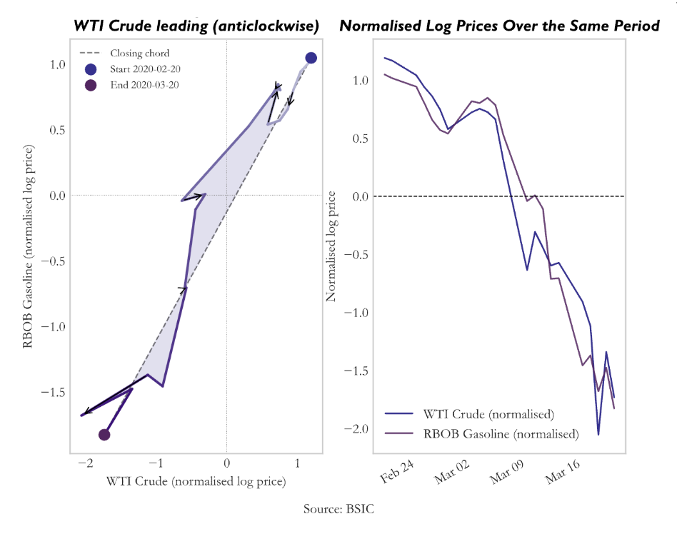
By applying the Lévy area to pairs of commodity price series, one can detect and quantify these lead–lag dynamics without pre-specifying their timing. A consistent sign in the Lévy area suggests that one market systematically moves ahead of another, providing a potential basis for forecasting and trading. In this sense, the Lévy area transforms geometric information about paths into economically meaningful signals, bridging advanced stochastic analysis with practical financial applications. By visualizing a short time-span example of the levy area on crude oil and gasoline, we can get:

Trade Idea 

For each trading day t, take the most recent W days of log prices (X, Y) and normalise both paths within the window. Then compute the discrete Stratonovich Lévy area (approximation of the integral). The intuition is mean-reversion on the laggard: if X has been leading Y, Y is expected to catch up. 

Entry: after EP (Entry persistence) + 1 consecutive days where the signal exceeds the threshold:

Exit: after XP + 1 consecutive days where the signal fades:

We justify EP (persistence) as one single day above the threshold is insufficient evidence of a genuine regime. A brief spike in the Lévy area could reflect a one-day price dislocation rather than a structural lead-lag shift. Without persistence, the strategy would frequently enter on transient spikes and reverse immediately. The exit is deliberately easier to trigger than the entry. Once the Lévy area drops below , the position is closed immediately.

We justify the magnitude of the signal = 1.5 as a signal of 1.5 means the joint path has traced a loop with sufficient area to be distinguishable from the noise envelope of a path with no lead-lag structure. Below this level, the directional signal is too weak relative to random path variation. The exit threshold is set to a lower requirement to prevent the strategy from repeatedly entering and exiting the same trade as the signal oscillates near a single threshold.

The window length is the most consequential parameter. Ten trading days corresponds to approximately two calendar weeks which is approximately the natural timescale for physical commodity adjustments. Crude oil refinery scheduling, crack spread realignments, and agricultural substitution all operate on weekly-to-fortnightly cycles. 

Note that all these assumptions are tested in-depth later in the article (statistical validation).

Crude to Gasoline

We begin with a canonical example: WTI crude oil and RBOB gasoline, a classic crack spread where economic structure strongly suggests lead–lag behaviour. Crude acts as the upstream input, while gasoline is a downstream refined product. Information shocks, inventory dynamics, and refinery constraints naturally create delays in price transmission.

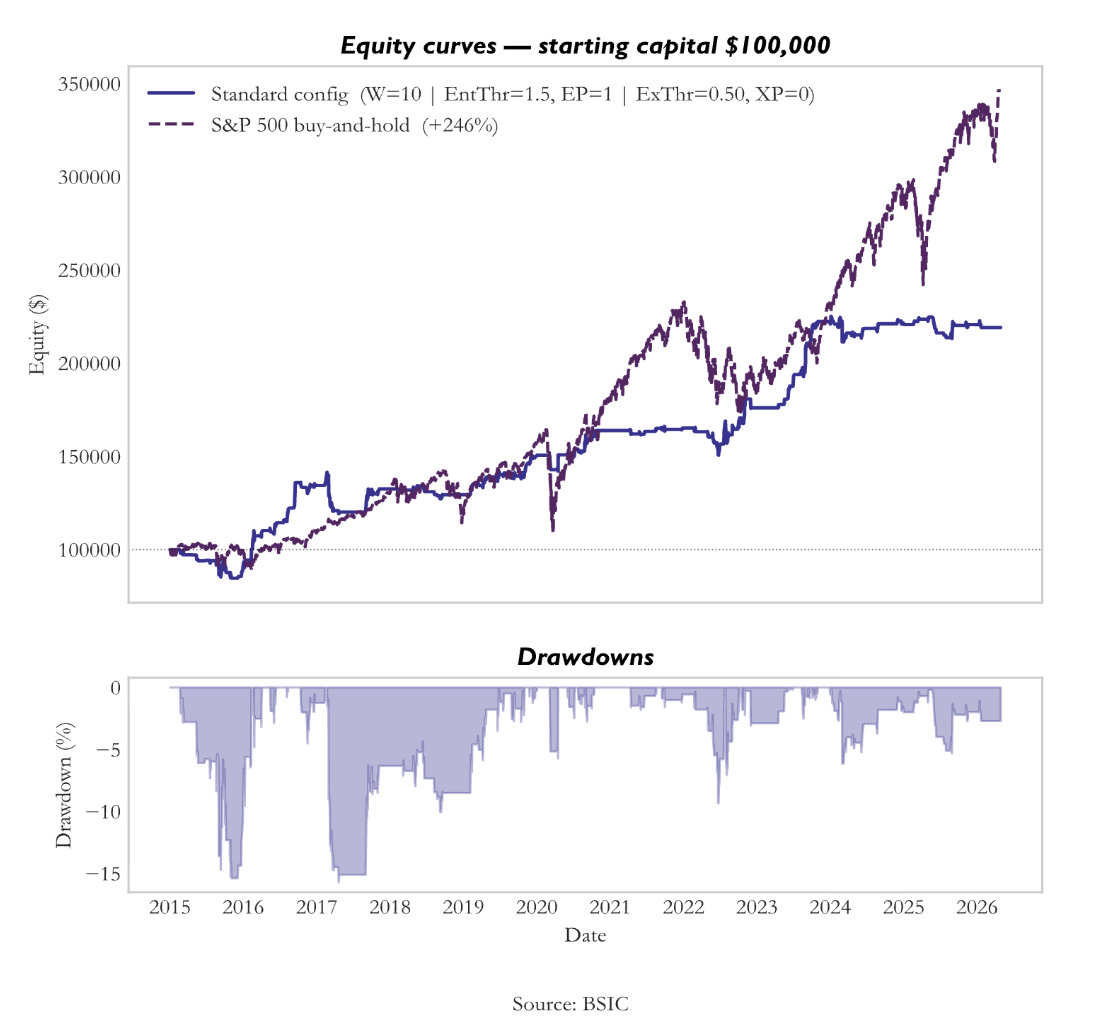
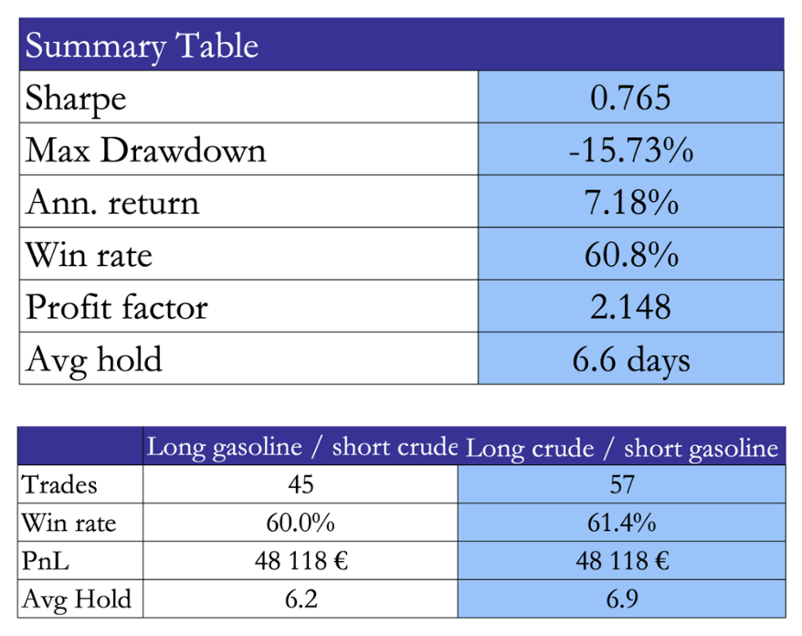
Portfolio Construction

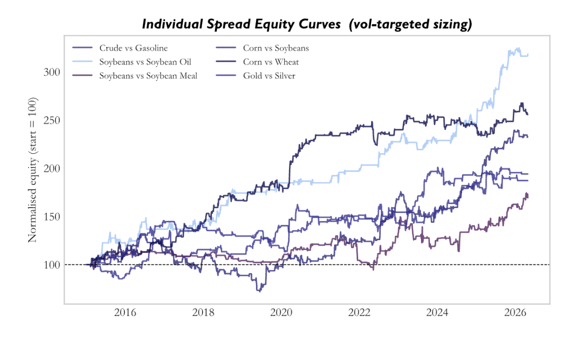
Having validated the strategy at the single-pair level, the framework is extended to a diversified portfolio of commodity spreads. The portfolio consists of six structurally motivated pairs:

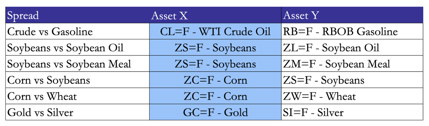These spreads are selected to capture economically grounded relationships where price dynamics are linked through either production chains or shared demand drivers. Vertical spreads such as crude to gasoline and soybeans to oil or meal reflect transformation processes, where upstream inputs influence downstream outputs with delays driven by processing and inventories. In contrast, horizontal spreads such as corn versus wheat or gold versus silver capture substitution effects and common macro drivers, where relative pricing adjusts as supply and demand conditions shift across closely related markets.

For each spread, the parameter configuration is specified ex ante based on a common baseline, taken as the configuration used for the Crude/Gasoline trade, which captures short-horizon lead–lag effects. Deviations are introduced only were justified by economic structure. For Soybeans vs Soybean Oil, the physical crush process operates on a slower 4–6 week cycle, so the window is extended to W = 30 to capture the full adjustment horizon. For Gold vs Silver where the relationship is heavily arbitraged and driven by institutional rebalancing over monthly horizons, the window is extended to W = 20 and the entry threshold increased to 2.0, ensuring that only strong and persistent signals survive arbitrage pressure.

Volatility scaling

Instead of trading fixed notionals, each position is scaled according to the recent realised volatility of the spread. At each point of entry, we compute the 20-day realized volatility of the spread return. A scaling factor is then applied, equal to the ratio of a target volatility level to the observed volatility, subject to upper and lower bounds:

Where is the realised standard deviation of the spread returns over the past 20 days, providing a measure of recent volatility. Target volatility is set to 3.5% per leg per day. Finally, this scaling factor is bounded by a floor and a cap to prevent extreme leverage or under-allocation

Transaction costs 

We assume a round-trip cost of 5 bps is applied at trade close on the full position notional.

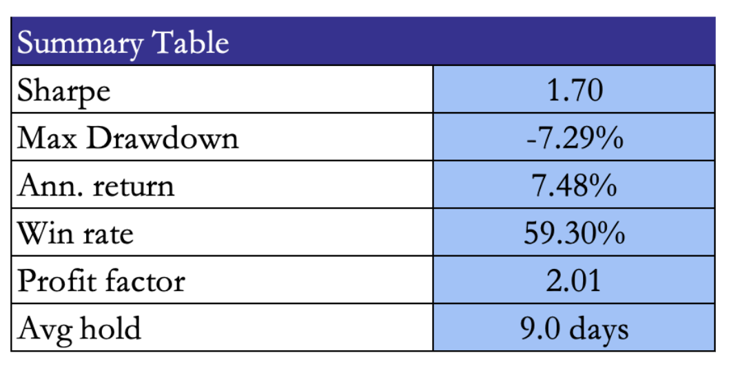
Results

Statistical validation

Firstly, we perform a permutation test, in which we take the actual trade structure, including the number of trades, holding periods, and volatility scalars per spread, but replace the Lévy area entry dates and directions with completely random ones, and run this process 1,000 times to build a null distribution of Sharpe ratios.

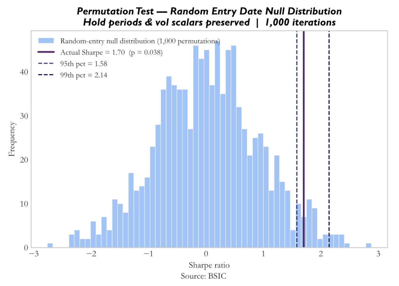The Lévy area is identifying genuinely better entry days than random. The specific timing of entries and not just the trade frequency or hold structure, is where the edge lives. That said, the p-value of 0.038 is significant but not overwhelmingly so.

Secondly, we conduct a walk-forward validation. The strategy is run from 2015 to 2020 with standard parameter modifications, then run from 2021 to the present with identical parameters.

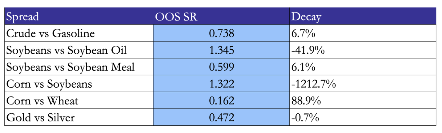
5 out of 6 spreads have OOS Sharpe > 0.5 which indicated that it is economically meaningful, thus the edge survives. Corn vs Wheat is the exception. It is strong in-sample, near-zero OOS. The grain substitution relationship likely shifted post-2020.

Risks and improvements 

The strategy carries several important risks that temper its results. Rolling window overlap creates mechanical clustering, meaning tests like runs and autocorrelation can overstate signal persistence and inflate statistical significance. There is also some parameter overfitting risk, such as the deviations applied to Soybeans versus Soybean Oil and Gold versus Silver, even if economically justified. In addition, the lack of a proper commodity factor benchmark means some of the measured alpha may reflect unmodelled exposures. Finally, the strategy does not scale cleanly, as larger capital allocations would likely face market impact and higher execution costs, especially in less liquid spreads.

Several improvements can enhance robustness and performance. A multi-window composite signal, combining Lévy area measures across different horizons such as 10, 20, and 30 days, would reduce sensitivity to any single parameter choice and improve signal reliability. The strategy can also be extended to new economically linked pairs across energy, metals, and soft commodities. Moving to intraday signal computation could improve Sharpe by enabling faster reactions and reducing holding risk. Transaction costs can further be reduced by batching trades across correlated spreads, such as executing shared legs only once when multiple signals trigger simultaneously.

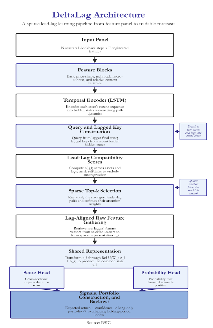
Model II: DeltaLag 

DeltaLag is designed to identify which assets systematically move before others. The architectural thesis is centered on a clear notion: the system is most effective when economic transmission is strong, cross-sectional redundancy is limited, and the training is rich enough to distinguish structure from noise. This is achieved by integrating four components:

1. Temporal encoding via Long-Short Term Memory (LSTM) that summarizes each assets price and feature history into a learned state space
2. Pairwise lag attention comparing the state of each asset to the lagged states of every other asset in the universe across specified timeframes.
3. Sparse leader extractor via top k attention selection to retain the most relevant relationships
4. Dual output heads that map information to an expected return and a directional probability score.

This design is intentionally more minimal than other computationally heavy systems. It has a small number of hidden dimensions, a single recurrent encoder, and a shallow score head. This aims to increase interpretability.

The LSTM Model

The first component of the DeltaLag architecture is an LSTM; this is a type of recurrent neural network designed to process sequential data one step at a time while carrying a hidden memory state forward. This is unlike a feedforward neural network which treats inputs as a single static vector. This accounts for the path dependence of asset pricing and risk distributions. However, a simple recurrent neural network (RNN) is insufficient; the system finds it difficult to preserve information across many time steps and signals quickly fade. As a result, an LSTM introduces an explicit memory cell and a set of gates, controlling what new information is added and should remain a part of the internal memory.

At each time step t, the LSTM receives three objects: the current input vector, the previous hidden state, and the previous cell state. The input contains the observed features at time t, such as returns, realized volatility, momentum measures, and other engineered characteristics. The hidden state is the model’s short-run summary of the sequence so far. The cell state is a more persistent memory channel designed to carry useful information across time.

First, the LSTM computes the forget gate. This determines how much of the previous memory should be kept. Since the sigmoid function maps into the interval (0,1), each element acts as a soft retention weight. Values near one preserve past information; values near zero suppress it. Second, it computes the input gate. This governs how much new information from the current time step should enter memory. Third, the model forms the candidate memory. This is the new content proposed for insertion into the cell state. It is constructed from the current input and the previous hidden state, then passed through a hyperbolic tangent so that the resulting values lie in (-1,1). This allows the candidate memory to encode both positive and negative contributions to the latent state.

These components are then combined in the cell-state update, where retained past memory and gated new information are merged into a single updated internal state. The output gate determines how much of this updated memory is exposed through the hidden state. In this sense, the cell state acts as the durable memory channel, while the hidden state is the filtered summary that is passed forward to later parts of the model. Economically, the purpose of this mechanism is to encode the recent path of the asset into a latent state that summarises its current condition. That state may reflect whether the asset is trending or mean-reverting, volatility is expanding or fading, price action is smooth or unstable, and whether the asset appears to be entering a breakout, rebound, compression, or stress regime.

The Transformer 

Readers familiar with modern deep learning will know that transformer architectures, built around self-attention, have become central in natural language processing and are increasingly used in finance. It is therefore useful to clarify how DeltaLag relates to that broader family of models. Although it is not itself a full transformer, it adopts the attention mechanism; it compares a current representation with a set of candidate representations, scorez their relevance, and aggregates information from the most relevant ones.

In a standard transformer, this operation is written as

The logic is straightforward. Queries represent what the current item is looking for, keys represent what each candidate item offers for comparison, and values are the information actually gathered once relevance has been established. The product QK computes similarity scores between queries and keys, the softmax transforms those scores into positive weights that sum to one, and those weights are then used to aggregate the values. In simple terms, attention asks which available information sources are most relevant to the current prediction, and how strongly each should influence it.

DeltaLag adopts this logic in a more economically specific way. It encodes each asset through an LSTM, which produces a hidden-state sequence summarising the asset’s recent trajectory. Attention enters after this temporal encoding stage. Its purpose is to identify delayed transmission channels across different assets. Fix one asset i, the asset whose current state we want to explain or forecast. DeltaLag treats this asset as the lagger. The LSTM has already produced its final hidden state, which summarises the recent temporal condition of that asset. This state is projected into the attention space to form a query. The query q_i can be interpreted as the pattern that asset i’s current state is searching for elsewhere in the market.

Now consider another asset j, treated as a potential leader. DeltaLag looks back over the recent encoded history of asset j and constructs a collection of lagged keys, one for each lag position in the recent window. The model is asking whether asset j at lag 1, lag 2, lag 3, and so on, matters for asset i now. Each candidate leader therefore contributes a bank of lagged reference states rather than a single static representation.

For each lagger the model computes a compatibility score. This dot product measures how strongly the current encoded state of asset i aligns with the lagged encoded state of asset j at a delay. A large positive score indicates strong alignment, a small score weak relevance, and a negative score poor alignment. Taken together, these scores define a three-dimensional search space over lagger, leader, and lag.

To prevent the architecture from collapsing into trivial own-series persistence, self-links are explicitly removed. After softmax, these entries receive zero weight. This forces the model to search for genuinely cross-asset predictive structure rather than simply rediscovering autoregression. DeltaLag also imposes sparsity. Instead of assigning positive weight to every possible leader–lag pair, it keeps only the top K scores for each lagger asset. These selected pairs define the active leader set for asset i at that moment. Their scores are then normalised through softmax to produce attention weights. This means the model proceeds in two stages: first, it decides which leader–lag relationships are worth keeping; second, it decides how much relative weight each selected relationship should receive. 

Finally, once the top K leader–lag pairs have been selected, DeltaLag gathers the corresponding raw lagged feature vectors from the original input representation. This produces the sparse relational representation for asset i. The choice to gather raw features rather than latent hidden states is deliberate. Hidden states are useful for matching because they summarise temporal patterns compactly, but they are also abstract and difficult to interpret economically. Raw features preserve direct financial meaning. DeltaLag therefore uses latent states to identify which relationships matter, but raw lagged observations to construct the final relational signal.

Dual Output Heads

After DeltaLag has gathered the most relevant lagged information from other assets, it combines that information into a single relational vector z_i for asset i. This vector is the weighted sum of the raw lagged features selected by the sparse attention mechanism. It therefore represents the cross-asset information the model has judged most relevant for forecasting asset i at that moment.

The model does not send z_i directly to the output layer. Instead, it first passes it through a shared feedforward transformation,

This produces a new internal representation u_i, which acts as a common state for the final prediction tasks. The purpose of this shared transformation is to reshape the gathered relational information into a form that is more useful for forecasting. In other words, z_i contains the selected market information, while u_i is the model’s refined summary of that information.

The nonlinearity here is the Rectified Linear Unit, or ReLU, which keeps positive values and sets negative values to zero. This matters because it makes the mapping from z_i to the outputs non-linear. Without it, the final stage would remain essentially linear and would be less able to capture more complex interactions among the gathered signals.

From this shared representation, DeltaLag produces two separate outputs. The first is the main forecasting output, or score head,

\hat{s}i = W{score} u_i + b_{score}

This produces a single scalar score for asset i. The score is the model’s primary signal and is intended to capture the asset’s relative attractiveness over the chosen forecast horizon. In a cross-sectional setting, this is fundamentally a ranking output. Assets with higher scores are interpreted as more attractive relative to the rest of the universe, while assets with lower scores are interpreted as less attractive. The score head therefore supports portfolio construction by ordering assets according to expected relative performance.

The second output is an auxiliary probability head. It first forms a logit from the shared representation and then maps it through a sigmoid function to produce a probability in the interval (0,1). This output can be interpreted as the estimated probability that the asset’s forward return over the forecast horizon will be positive. The distinction between the two heads is important. The score head learns relative expected return; the probability head learns directional likelihood. 

Feature Set, Parameters and Training

The input to DeltaLag is a rolling panel of assets. At each date, the model observes the full universe over a recent lookback window, so the data can be viewed as a three-dimensional object: number of assets, number of time steps, and number of features per asset. In the reference configuration, the lookback window is typically about 60 trading days and the feature set contains roughly 20 engineered variables per asset

The feature design is modular. Rather than relying on one undifferentiated block of predictors, DeltaLag uses several feature families, each intended to describe a different aspect of market behaviour. The first contains basic price-shape and activity variables, such as one-day returns, volume, turnover, and intraday location measures based on the open, close, high, and low. These describe whether the asset trended, reversed, or traded with unusual participation over a very short horizon. A second family contains more explicitly technical variables, including cumulative returns over several horizons, moving-average gaps, and rolling volatility. A third family adds macro-context variables, which are especially useful when the universe includes macro anchors such as the dollar, volatility, rates, credit, or gold. A fourth family adds relative-context variables, which are particularly important in a cross-sectional setting because they describe how an asset is behaving relative to the market and relative to the rest of the universe.

The core model parameters are conservative. The preferred configuration uses a hidden dimension of 32, a single LSTM layer, and sparse top-k attention with k=3. The shared feedforward layer is also kept small, and dropout is modest rather than aggressive. Training is carried out one horizon at a time. The relevant transmission channels, persistence of leadership, and economic mechanisms may differ materially across horizons. Shorter horizons may reflect faster rotation and flow-based effects, while longer horizons may capture slower macro adjustment or sector transmission. By training separate models, DeltaLag avoids forcing structurally different problems into one common parameter set.

The main loss is applied to the score head, typically using Huber loss on the cross-sectional z-scored forward return. Huber loss is useful because it behaves like squared error for small residuals but becomes linear for larger ones, making it more robust to the heavy tails and occasional large moves common in financial data. The probability head is trained in parallel using binary cross-entropy on the directional label. The two losses are combined in a multi-task objective, with the ranking task treated as primary and the directional task as an auxiliary source of supervision.

Optimisation is performed with AdamW, which combines adaptive learning rates with decoupled weight decay. In practice, this helps the model converge more stably while discouraging excessively large parameter values that would be suggestive of overfitting. Gradient clipping is used to control recurrent training instabilities, especially exploding gradients, and a learning-rate scheduler reduces the step size when validation performance stops improving. The base learning rate is deliberately conservative because in low-signal financial settings large learning rates often produce instability rather than genuine discovery. Training is also controlled by early stopping, with the best checkpoint selected according to validation information coefficient rather than raw loss.

Portfolio Construction and Backtesting

Once DeltaLag has generated daily forecasts, the next task is to convert those model outputs into tradeable portfolio signals and to evaluate them in a systematic backtest. The starting point is the model’s inference output. For each date, asset, and forecast horizon, DeltaLag produces a score, a raw score output, and a probability that the asset’s forward return will be positive. The model also records the selected leaders, lag positions, and attention weights, the prediction file contains not only a final forecast but also the relational structure behind that forecast. These raw outputs are then transformed into a signal table. The score is re-normalised cross-sectionally within each date and horizon to form an expected-return signal. 

At the same time, additional quantities are constructed that help describe the conviction of the forecast. One is attention concentration, which measures whether the model’s prediction is dominated by one leader or spread across several. Another is directional confidence, derived from how far the probability estimate lies from an even fifty-fifty outcome. These are combined into a broader confidence measure, so that each forecast is represented not only by its expected return ranking, but also by the degree of structural conviction behind it.

From this signal table, DeltaLag supports a long-only portfolio. On each signal date, the model looks across all assets within a given horizon and keeps only those with positive expected-return forecasts. Among these, it selects the top K assets with the largest expected-return values. These selected assets become the constituents of a new long book opened on that date. The portfolio is not equally weighted by default. Instead, weights are based on the magnitude of the expected-return signal itself. Assets with larger positive expected-return scores receive larger weights, although the weights are capped by a maximum position size so that no single asset can dominate the book. After this cap is applied, the weights are re-normalised so that they again sum to one. In this way, the long-only portfolio remains concentrated in the strongest signals, but still subject to basic diversification control.

Once the daily books have been formed, the backtest uses an overlapping holding-period structure. The model may generate a forecast every day, but the forecast horizon itself may be ten days, twenty days, or some other multi-day interval. If positions were opened and closed fully every day, the implementation would not match the horizon embedded in the target construction. DeltaLag therefore holds each newly formed book for a horizon-specific number of trading days. On any given day, the active portfolio is the average of all books that were opened on earlier dates and whose holding periods have not yet expired. In other words, several books initiated on different dates can coexist at the same time, each still contributing to the current portfolio return. This produces an overlapping-book structure that is much closer to how medium-horizon forecasts would be expressed in an actual trading process.

The long-only backtest computes returns by tracking the next-day price change of every asset currently held in each active book. For each sub-book, the weighted average return of its constituent assets is computed using the portfolio weights assigned at entry. If multiple books are active on the same date, their returns are averaged, producing the daily return of the overall long-only strategy. 

Transaction costs are incorporated in a simplified way. Rather than modelling individual execution slippage trade by trade, the framework applies a transaction-cost penalty measured in basis points. This cost is subtracted as an entry-cost proxy, spread over the holding window of the position. The purpose of this adjustment is to ensure that the backtest does not treat all rebalancing as frictionless. Since the strategy can open new books frequently, especially when signals are generated daily, this transaction-cost term is necessary to give a more realistic measure of net performance.

After the daily return series have been computed, the backtest builds cumulative return paths horizon by horizon. Standard performance summaries can then be calculated from these daily returns, including mean return, volatility, Sharpe ratio, and maximum drawdown. Importantly, however, the conceptual role of the backtest is to test whether the signal-construction and portfolio-formation logic work coherently when embedded in a realistic holding-period framework. 

Results Overview

The 20-day horizon performs strongly across every major dimension examined: training behaviour, validation IC, signal quality, network structure, portfolio composition, and realised backtest path. The 10-day horizon, by contrast, underperforms persistently, and the diagnostics make clear that this weakness is not incidental. It is traceable to unstable learning, weaker signal persistence, heavier concentration on a small set of leaders, and an inability to convert learned structure into robust out-of-sample returns. 

Loss Curves and Convergence

The 10-day model is trained using binary cross-entropy over cross-sectionally standardised excess-return targets, with a learning rate held at 0.0003 through most of training and only reduced at the end. Its loss path appears superficially well behaved on the training set, declining from 0.632 to 0.466, but the validation trajectory is much less reassuring. Validation loss bottoms near epoch 8, around 0.498, and then rises again, reaching roughly 0.506 by epoch 12. This is the familiar signature of a model that can fit the training sample but cannot maintain generalisation. The best checkpoint is saved earlier, at epoch 6, where validation IC reaches 0.0207. 

The 20-day model behaves differently. Here the training loss declines from 0.814 to 0.449 over a longer and more disciplined training path, while the learning rate is cut at epoch 8 and then again to later in training. Validation loss falls more smoothly, reaching its minimum near epoch 12, around 0.513, and remaining relatively stable thereafter. The best checkpoint is saved at epoch 12 with validation IC of 0.0667. The tighter alignment between train and validation trajectories, together with the more orderly learning-rate schedule, suggests that the 20-day model is discovering a richer and more persistent cross-sectional signal. 

Validation IC Evolution

The validation IC curves make the divergence even more explicit. The information coefficient is the cross-sectional correlation between the model’s predicted rankings and the realised future returns. At the 10-day horizon, IC oscillates violently between negative and weakly positive values, ranging from roughly -0.042 to +0.021, with no stable upward trend. The best reading occurs at epoch 6 and is then followed by a rapid deterioration. This is the profile of a model briefly discovering a local pattern and then losing it as parameter fitting continues. Since validation IC, rather than raw loss, is the economically relevant metric in a ranking architecture, this instability is especially damaging: the model may continue optimising, but it is not improving in the sense that matters for portfolio formation.

The 20-day IC curve is materially stronger. It begins in positive territory, dips briefly, and then rises through the lower-learning-rate phase to a peak of 0.0667 at epoch 12. This is more than three times the 10-day peak. More importantly, it reflects a coherent training narrative: once the model enters the lower-learning-rate phase, its ranking ability improves rather than destabilises. Since DeltaLag selects checkpoints using validation IC rather than loss, this pattern is exactly what one would want to observe in a research setting focused on cross-sectional ordering. 

Prediction Dispersion

Prediction dispersion provides an additional lens on model quality. A ranking model that collapses to near-constant predictions cannot generate useful portfolio signals. At the 10-day horizon, the standard deviation of cross-sectional predictions falls from 0.016 at epoch 1 to values around 0.004–0.007 during the early-middle phase of training, before expanding sharply to 0.044 later on. This sequence is diagnostic of a weak model state: first compression toward an uninformative constant output, then noisy re-expansion as overfitting sets in. It is therefore not surprising that the 10-day model ultimately struggles out of sample.

The 20-day model again shows the healthier profile. Dispersion begins around 0.024 and rises in a broadly monotonic fashion toward 0.059 by the late epochs. This implies that the model is progressively sharpening its cross-sectional differentiation without collapsing. Out of sample, both horizons retain properly standardised signal distributions, with signal means effectively at zero and standard deviations near one, but the training path matters: the 20-day model reaches its final dispersion through controlled learning, while the 10-day model reaches it through instability. That distinction becomes important later when interpreting why one horizon generates profitable books while the other does not.

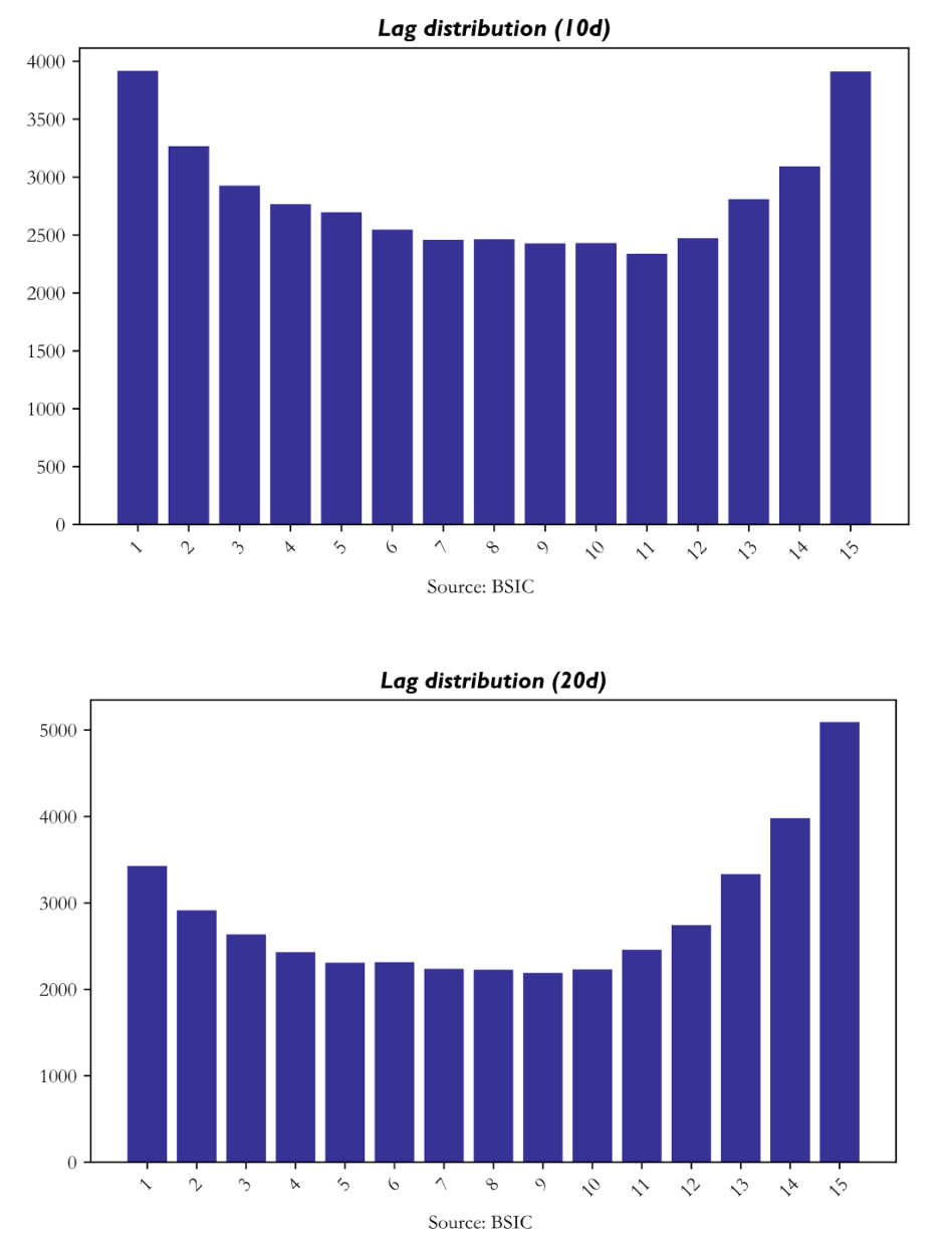
Lag Distribution

The lag-distribution results are among the clearest windows into what the model is learning. Across both horizons, the selected lag positions are concentrated at the very short end of the search window, especially lag 1, and then again toward the far end, particularly around lags 13–15. At the 10-day horizon, lag 1 is selected 3,918 times and lag 15 3,912 times. At the 20-day horizon, lag 1 appears 3,428 times, but lag 15 rises much more strongly, reaching 5,093 selections. 

This pattern is economically meaningful. The mass at lag 1 captures fast information diffusion: market leadership that propagates within a day or within the next weekly block of trading. The secondary mass at lags 13–15 reflects slower propagation: multi-week momentum, delayed macro transmission, or cross-sector adjustment processes that require more time to appear in returns. The 20-day model leans more heavily into these longer-end lags. It suggests that the monthly-horizon signal is drawing more heavily on a slower and more persistent relational structure. The resulting U-shaped lag profile is therefore one of the strongest pieces of evidence that DeltaLag is learning structure rather than a conventional short-term cross-sectional momentum effect.

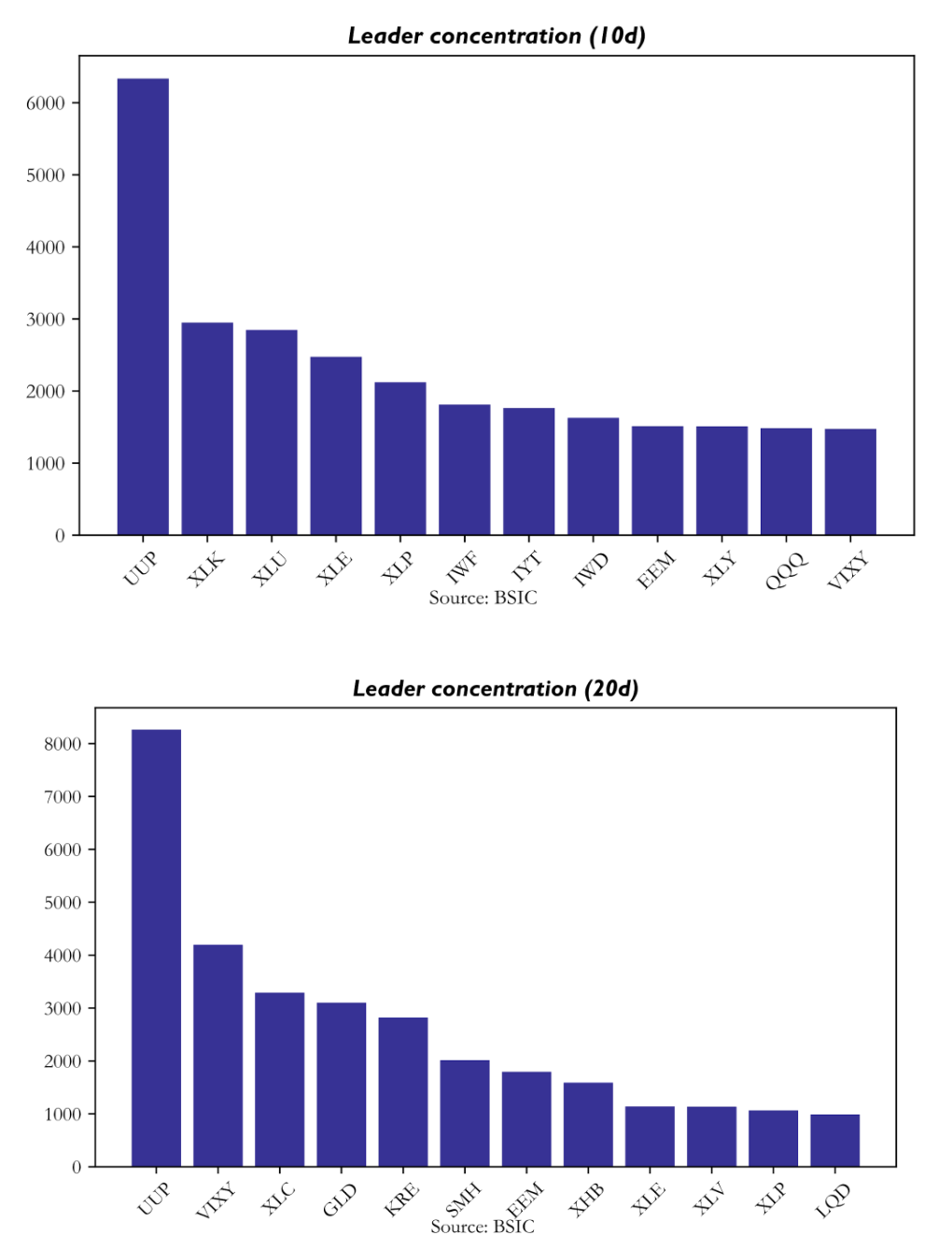
Leader Concentration

Leader concentration reveals which assets repeatedly serve as informative anchors for the rest of the universe. Across both horizons, the single dominant leader is UUP, the U.S. dollar proxy. At the 10-day horizon it is selected 6,335 times; at the 20-day horizon that rises to 8,263. This means the model is repeatedly identifying the dollar as the most informative upstream node in the network. At 10 days, the next most common leaders are XLK, XLU, XLE, and XLP. At 20 days, the hierarchy shifts materially: UUP remains first, but it is followed by VIXY, XLC, GLD, and KRE. 

This leader structure is one of the strongest validations of the model’s economic interpretability. UUP makes sense as a universal macro anchor because dollar strength conditions risk appetite, commodity pricing, international equity sensitivity, and sector rotation. The rise of VIXY at the 20-day horizon is equally meaningful: it suggests that volatility regime matters more for medium-horizon returns than for shorter tactical ones. Likewise, the importance of GLD and KRE indicates that gold and regional banks become informative state variables once the horizon is long enough for risk-regime adjustment to work through the system. Crucially, the network does not collapse entirely into one or two nodes. Although UUP dominates, all 32 assets appear as leaders with non-trivial frequency, and the overall persistence score remains around 0.527 with low dispersion. That means the graph is sparse but not frozen: structured enough to be interpretable, yet dynamic enough to adapt through time.

Highest-Conviction Lead–Lag Pairs

The highest-conviction pairwise relationships further clarify what the model regards as economically actionable. At the 10-day horizon, the strongest pair is XLK leading XLE at lag 1, with flow strength 2.466. UUP leading IWF is second, followed by QQQ leading XLC. These are plausible short-horizon leadership channels: technology into energy, dollar into growth, broad large-cap tech into communications. Yet they are also unstable in aggregate, as reflected by the weak backtest that results when these signals are converted into a long-only book.  

At the 20-day horizon, the most powerful pairs are more clearly macro-regime oriented. UUP leads QQQ, UUP leads IWM, VIXY leads IWM, VIXY leads IYT, and XHB leads XLU. The repeated appearance of XHB with XLU with persistence near 0.816 is particularly telling, since it suggests a stable rate-sensitive cross-sector channel. This is exactly the kind of sparse but recurring graph that DeltaLag was designed to expose: not a dense matrix of weak correlations, but a small set of temporally displaced relationships with repeatable economic interpretation.

Cross-Sectional Signal Properties

The full signal table contains 28,352 observations, split evenly across the two horizons. Several features of the signal distribution are immediately reassuring. First, both horizons remain well centred, with signal means effectively at zero. This confirms that the cross-sectional normalisation is functioning correctly and that the system does not carry a mechanical directional bias. Second, signal standard deviations remain near one, again consistent with correct scaling. Third, the 20-day horizon exhibits a higher mean probability of positive return, 0.683 versus 0.654 for the 10-day model, which is broadly consistent with the stronger realised long-only performance. 

Another important difference lies in attention concentration. At the 10-day horizon, the primary leader captures about 49.9% of total attention weight on average. At the 20-day horizon, that falls to 39.8%. This is a subtle but important result. The shorter-horizon model is more concentrated on one dominant explanatory channel, usually UUP, whereas the longer-horizon model distributes its explanatory mass more broadly across multiple leaders. This diversification of explanatory structure likely contributes to the improved robustness of the 20-day signal. A more diversified attention map is less vulnerable to the failure of any single macro channel and more consistent with a stable portfolio signal.

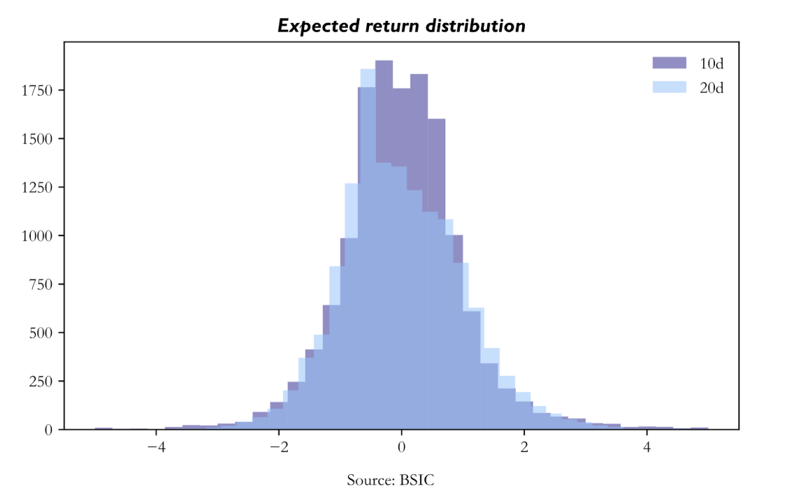
Expected Return Distribution

The expected-return distributions also differ in an economically meaningful way. Both are symmetric and centred near zero, but the 10-day distribution is more sharply peaked around the centre, while the 20-day distribution is broader with heavier tails. Put differently, the 20-day model generates more extreme positive and negative cross-sectional views, while the 10-day model is more compressed. This matters because a long-only portfolio built from top-ranked assets benefits when the signal can separate the strongest opportunities more decisively. The broader 20-day distribution therefore translates naturally into more concentrated and more profitable selections. The top expected returns in the 20-day portfolio are indeed somewhat higher on average, and the holdings summary confirms that the average expected-return signal among top-held assets is stronger at 20 days than at 10 days.

Backtest Performance

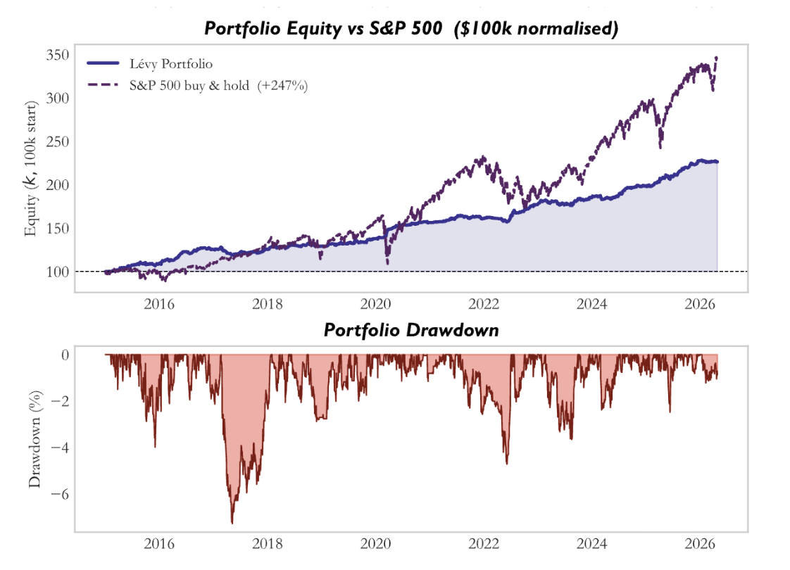
At the 20-day horizon, the strategy generates a total return of 32.03% over 22 months, with daily volatility 0.684%, annualised Sharpe 1.514, rolling Sharpe mean 1.799, rolling Sharpe median 2.166, and maximum drawdown -7.29%. The strategy is profitable in 14 of 22 months, with its best month at +9.01% and its worst month at -5.19%. These are strong results not only in absolute terms but also in path quality. The return path is profitable, the Sharpe is decisively positive, and the drawdown is modest relative to the level of return generated.

The 10-day strategy, in contrast, is weak across nearly every metric. Total return is -3.24%, mean daily return is slightly negative, annualised Sharpe is -0.131, and maximum drawdown reaches -17.67%. Although the rolling Sharpe median is positive, the mean remains negative because a number of severe downside episodes dominate the distribution. The strategy is positive in only 11 of 22 months. This is not the profile of a merely mediocre signal. It is the profile of a signal that occasionally works but is too unstable to survive implementation in a repeated overlapping-book process. Table 8 states this divergence very clearly, and it is one of the decisive results of the paper.

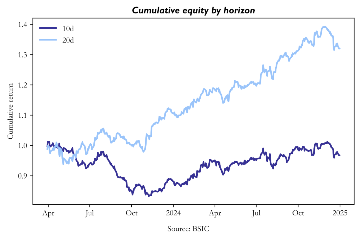
Cumulative Equity Curves

The cumulative equity curves make the difference intuitive. The 20-day strategy rises from 1.000 to a peak near 1.392 and ends at approximately 1.320. The path is not perfectly smooth, but it is recognisably upward sloping and contains recoverable pullbacks rather than structural collapse. The 10-day path, by contrast, spends most of the sample below par, falls to a trough near 0.833, recovers only partially, and ends at 0.968. The visual implication matches the summary statistics: the 20-day model compounds, the 10-day model struggles.

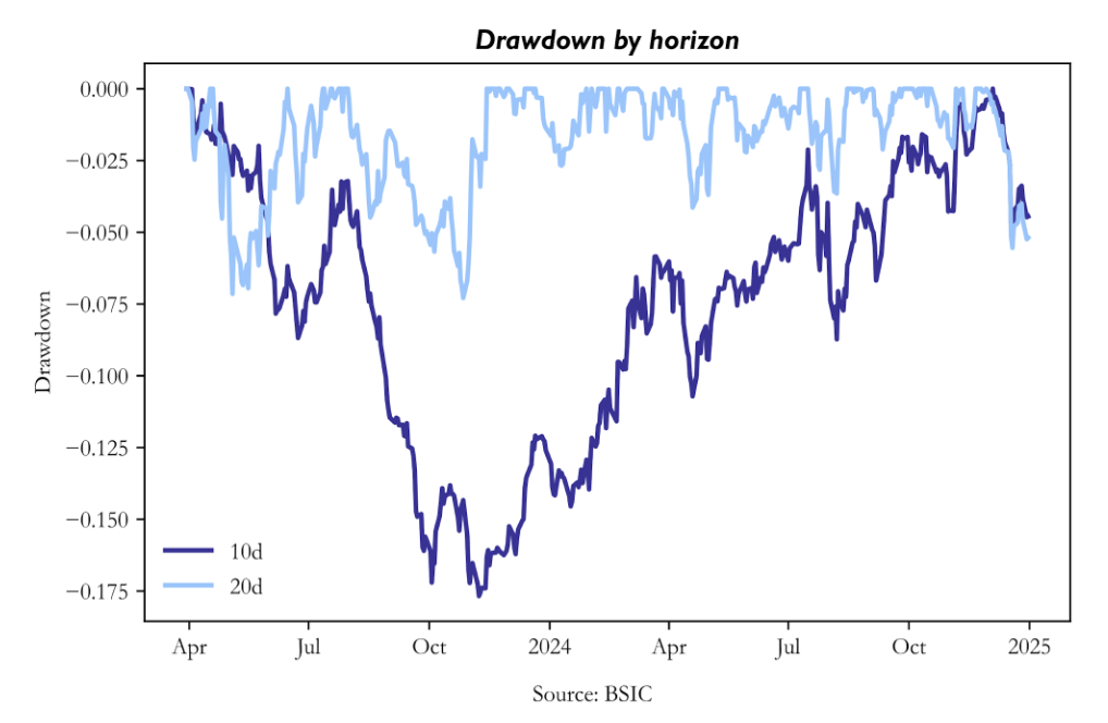
Drawdown Analysis

Drawdown analysis strengthens the same conclusion from the risk side. The 10-day strategy experiences a long and deep drawdown, reaching -17.67%, and spends an extended period below -5%. It is evidence that the underlying signal is too weak to support repeated long-only deployment at this horizon. The 20-day strategy’s worst drawdown, by contrast, is only -7.29%, and its average drawdown is much smaller. The resulting profile is consistent with a strategy that has genuine positive expected value but is subject to ordinary market variation rather than structural failure.

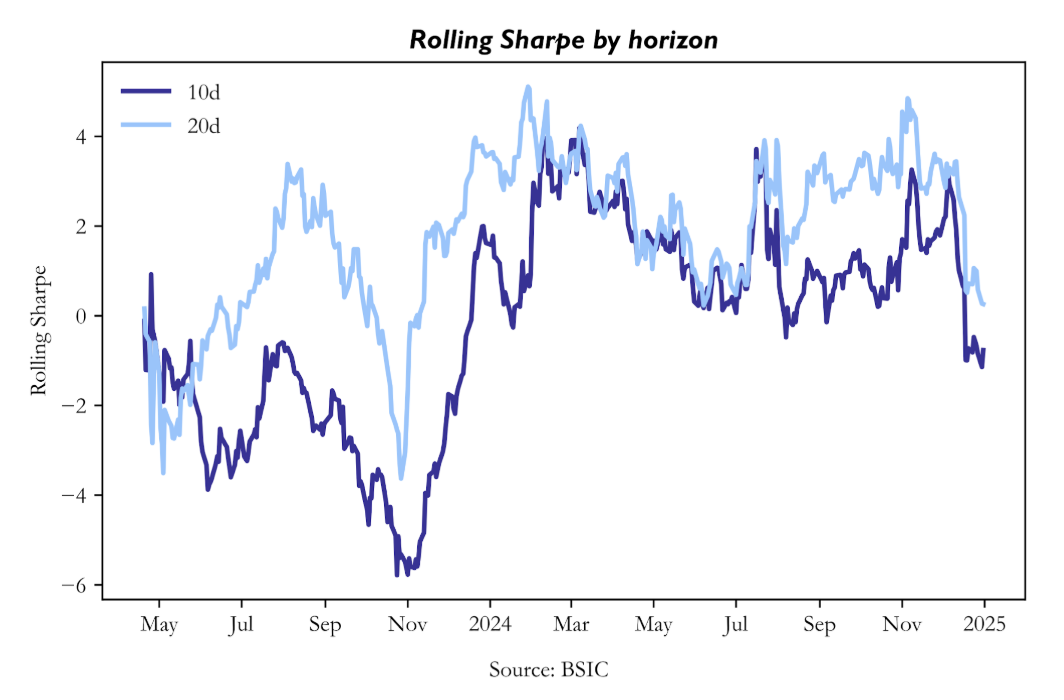
Rolling Sharpe Ratio

The rolling Sharpe chart adds temporal resolution. The 20-day strategy maintains a predominantly positive rolling Sharpe across most of the evaluation window, with a mean of 1.799 and a median of 2.166. This matters because it demonstrates that the strategy’s positive performance is not concentrated in one short episode. By contrast, the 10-day rolling Sharpe oscillates around zero, with a negative mean and occasional sharp negative spikes. This pattern is exactly what one would expect from a model that intermittently captures directional structure but cannot hold it consistently enough to sustain a robust strategy path.

Monthly Return Attribution

The month-by-month return table provides a final layer of texture. The 10-day strategy’s worst months, August and September 2023, coincide with a broader risk-off episode associated with rising real yields and dollar strength. The 20-day model handles those same conditions far better, suggesting that its broader leader set, especially the inclusion of VIXY and other macro-sensitive channels, provides a more resilient mapping from regime information to portfolio positioning. Likewise, the 20-day model’s strongest months, notably November 2023 and July 2024, align with broad equity rallies in which cyclical exposure and macro-sensitive sector leadership were rewarded. The 10-day strategy participates in those rallies, but much more weakly. Across the 22-month window, the 20-day model outperforms the 10-day model in 17 months on a raw-return basis. That is too persistent a pattern to dismiss as luck.

Universe Design and Prior Comparisons

Futures-heavy sleeves generally underperformed because carry, roll, and the heterogeneous structure of commodity markets weakened the clean cross-sectional object that the model expects. Single-equity universes also underperformed, but for the opposite reason: they lacked the sector-factor architecture that makes leader–lagger relationships both stable and interpretable. By contrast, the ETF universe succeeds because it preserves economically meaningful transmission channels while remaining sparse enough for top-k attention to identify useful leaders.

Across the broader experimental programme, one conclusion was especially clear: universe design mattered more than brute-force model complexity. The strongest performance did not come from the broadest or most elaborate basket but rather the universe that combined economic coherence with manageable graph density.

The semiconductor and infrastructure supply-chain sleeve was the strongest thematic alternative. It produced long-only Sharpe ratios of roughly 1.34 at 10 days and 1.22 at 20 days, confirming that DeltaLag can work well in a thematically coherent universe when the underlying economic logic of delayed transmission is strong. However, it remained narrower and more theme-dependent than the compact macro-sector winner. As a result, it generated good alpha, but not the same breadth of persistent macro and cross-sector transmission.

The extended sector/subsector ETF basket performed respectably, but it was not optimal. Its best expression was long-only at the 20-day horizon, with Sharpe around 1.18. This is a solid result in isolation, but clearly weaker than the compact winner. The most likely reason is graph dilution. Adding more sector and subsector ETFs broadened the internal rotation graph, but did not add enough genuinely new information per node. Instead, the universe became crowded with overlapping and correlated sleeves. For a sparse relational model, this is exactly the kind of environment that weakens performance: the model sees more apparent leaders, but too many of them are redundant.

The ultra-core macro transmission sleeve underperformed for the opposite reason. Where the extended ETF basket was too broad, the ultra-core sleeve was too narrow. By removing too many nodes, it cut off useful transmission channels and stripped away intermediate state variables that helped the winning sleeve function. In practical terms, this test confirmed that cleaner is not always better. Beyond some point, simplification stops removing noise and starts removing structure.

Potential Improvements and Next Research Directions

The current results suggest that the next stage of development should focus on sharpening the parts of the system that already work, especially the 20-day horizon. The evidence indicates that DeltaLag is strongest when it captures medium-horizon macro and sector rotation, so future work should treat that horizon as the core research object rather than as one candidate among many. The 10-day model is useful as a comparison, but the 20-day system appears to be the natural expression of the architecture in the present ETF universe.

A first improvement is more explicit horizon specialization. At present, the same general architecture is used across both horizons, even though the diagnostics suggest that the underlying transmission structure differs materially. A better approach would be to optimize the 20-day model specifically for slower macro-sector rotation: longer-horizon features, stronger emphasis on persistence, and portfolio rules designed for medium-term repositioning rather than shorter tactical moves. In practice, this means treating the current 20-day system as the base model and refining around it.

There is also room to improve the machine-learning architecture itself. The current model is intentionally small and sparse, which is one of its strengths, but several extensions are plausible. The first is better lag design. The diagnostics show meaningful mass at both lag 1 and the far end of the lag window, especially around lags 13 to 15. Rather than searching over a flat lag bank, the model could use grouped lag regimes, for example short, medium, and long lags. This would make the temporal structure easier to learn and easier to interpret. 

Second, sparsity itself could become adaptive. A fixed top-k is useful, but different regimes may require different active neighbourhood sizes. A more flexible sparse-attention rule could improve robustness without sacrificing interpretability. Third, the dual-head structure could be used more effectively in downstream portfolio construction. At present, the score head dominates. Future versions could make more direct use of the joint information in score, probability, and attention concentration.

Training can also be improved. The current results show that the 10-day model suffers from unstable convergence, while the 20-day model benefits from a cleaner learning path. This suggests a need for stronger horizon-specific training discipline. More aggressive early stopping, better calibration of learning-rate decay, and more systematic hyperparameter selection around validation IC would likely improve reliability. The 10-day results also suggest that prediction collapse and later overfitting remain real risks. Additional regularisation, stronger dropout tuning, or explicit penalties against low-dispersion predictions may help prevent this. More broadly, the model should continue to be judged primarily by validation IC and out-of-sample ranking performance rather than by raw training loss.

Feature design is another obvious area for improvement. Since the strongest leaders at the 20-day horizon are macro anchors such as UUP, VIXY, GLD, and KRE, the feature space should be expanded in a way that helps the model describe macro state more precisely. This does not mean adding features indiscriminately. It means adding features that sharpen the regime dependence of the graph: richer credit-spread information, volatility-state measures, rates-sensitive relative performance, and stronger relative-strength features across sectors and factors. The current model already learns macro structure from price histories alone; a better state description should help it do so more consistently.

Portfolio construction could also be improved substantially. The current overlapping long-only book proves that the signal survives implementation, but it is still a relatively simple expression of the forecasts. Better turnover control, volatility-aware sizing, and more refined holding-period management could all improve realised Sharpe. More importantly, the architecture is fundamentally relative in nature. Even when run as long-only, it is selecting relative winners. That suggests future versions may be even stronger in a long-short, market-neutral, or long-underweight framework, where the ranking signal can be expressed more directly.

Conclusion

Lead–lag structure is a family of delayed transmission relationships whose usefulness depends on the market, the horizon, and the modelling framework used to detect them. This article examined two very different approaches to that problem. The Lévy area offered a geometric, path-wise method for extracting directional asymmetry from commodity spreads and showed that economically grounded pair relationships can be translated into systematic trading signals. DeltaLag, by contrast, approached the same problem through a sparse machine-learning architecture designed to identify which assets lead others, at which lags, and with what forecasting value.

The central empirical result is that the success of lead–lag modelling depends less on raw model complexity than on whether the structure being modelled is economically coherent. In the commodity setting, the Lévy area worked best when applied to spreads supported by clear production-chain or substitution logic. In the cross-asset ETF setting, DeltaLag worked when the universe contained interpretable macro and sector transmission channels and when the forecast horizon was long enough for those channels to propagate. The strongest DeltaLag result emerged at the 20-day horizon, where the model produced superior validation IC, more stable leader structure, broader relational support, and a materially stronger long-only backtest than the shorter-horizon alternative.

References

[1] Bouchouev, Ilia, “Virtual Barrels, Quantitative Trading in the Oil Market”, 2023.  

[2] Zhou, Wanyun, Wang, Saizhuo, Cucuringu, Mihai, Zhang, Zihao, Li, Xiang, Guo, Jian, Zhang, Chao, and Chu, Xiaowen, “DeltaLag: Learning Dynamic Lead-Lag Patterns in Financial Markets”, 2025.  

[3] Wang, Saizhuo, Kong, Hao, Guo, Jiadong, Hua, Fengrui, Qi, Yiyan, Zhou, Wanyun, Zheng, Jiahao, Wang, Xinyu, Ni, Lionel M., and Guo, Jian, “QuantBench: Benchmarking AI Methods for Quantitative Investment”, 2025.  

[4] Bennett, Stefanos, Cucuringu, Mihai, and Reinert, Gesine, “Lead–lag Detection and Network Clustering for Multivariate Time Series with an Application to the US Equity Market”, 2022.  

[5] Zhang, Yichi, Cucuringu, Mihai, Shestopaloff, Alexander, and Zohren, Stefan, “Dynamic Time Warping for Lead-Lag Relationship Detection in Lagged Multi-Factor Models”, 2023.  

[6] Shi, Danni, Calliess, Jan-Peter, and Cucuringu, Mihai, “Multireference Alignment for Lead-Lag Detection in Multivariate Time Series and Equity Trading”, 2023.  

[7] Hochreiter, Sepp, and Schmidhuber, Jürgen, “Long Short-Term Memory”, 1997.  

[8] Vaswani, Ashish, Shazeer, Noam, Parmar, Niki, Uszkoreit, Jakob, Jones, Llion, Gomez, Aidan N., Kaiser, Łukasz, and Polosukhin, Illia, “Attention Is All You Need”, 2017.  

[9] Li, Yuncheng, Song, Yale, and Luo, Jiebo, “Improving Pairwise Ranking for Multi-Label Image Classification”, 2017.  

[10] Zhong, Jianyuan, Xu, Zhijian, Wang, Saizhuo, Wen, Xiangyu, Guo, Jian, and Xu, Qiang, “DSPO: An End-to-End Framework for Direct Sorted Portfolio Construction”, 2024.