Introduction on TIPS and Gold as inflation hedge
Generally, an assets is considered t o be an “inflation hedge” if either its purchasing power is maintained over the long run or its nominal returns closely track realized inflation over shorter horizons. Gold and TIPS fall into this category and are thus correlated given that they become more desirable to hold under similar conditions. Regardless, the two assets have different characteristics and they hedge inflation in a different manner.
Treasury inflation protected securities (TIPS) refer to a treasury security that is indexed to inflation in order to protect investors from the negative effects of inflation. TIPS are considered an extremely low-risk investment since they are backed by the U.S. government and because the par value rises with inflation, as measured by the Consumer Price Index, while the interest rate remains fixed. For this reason, TIPS can be classified as indexed-bonds where the final payment rather than the coupon rate is adjusted for CPI inflation.
Buying a TIPS means basically securing the real yield conditionally on holding the bond until maturity: this is due not only to the basic concept of yield to maturity but also it is a consequence of the fact that coupon rate is not adjusted, rather principal payment is corrected for inflation.
A final note on TIPS: not all of them are born equal! In a paper by Vanguard (“The Long and Short of the TIPS, October 2012), it is shown that the return on a short-term TIPS benchmark (of 0-to-5-year maturities) has been more highly correlated to actual monthly and yearly CPI (Consumer Price Index) inflation than other segments of the U.S. TIPS market over the past decade. Although, in practice, all TIPS securities receive the same CPI principal adjustment, short-term TIPS returns tend to most closely track actual CPI inflation because of their lower duration and greater responsiveness to temporary, unexpected inflation spikes. Indeed, TIPS, especially with shrorter maturities, are thus more reactive to inflation expectations.
On the other hand, Gold is widely viewed as a hedge against long run inflation. In fact, the effectiveness of gold as a hedge against inflation seems somewhat controversial for short- and medium-term horizons. Moreover, the most reliable relationship exists between gold and strong increases in inflation, while moderate increases in inflation or declining inflation do not materially impact the price of gold in either direction. Nonetheless, when inflation runs out of control, gold tends to benefit significantly and to outperform other hedges against inflation. In addition to this, it looks that some gold investors fail to consider its volatility as well as its opportunity cost, while others fail to anticipate storage needs and other logistical complexities of gold ownership. Meanwhile, slow but steady, Treasuries provide less excitement but reliable income. And the longer the gold is held over Treasuries, the more painful these opportunity costs can become, due to sacrificed compound interest.
The strong historical correlation between the two and their recent divergence
The relationship between these two safe havens diverged substantially over the last six months compared to the period before where the two series had been moving together. Since both assets are considered a natural hedge against inflation, they should theoretically be strongly correlated: when gold goes up the yield of the tips should go down (or up in this inverse chart). Instead this is not really the case, given that the gold price rise while yield rose, i.e. TIPS bond prices down meaning that they are less desired.
A possible explanation could be related to the fact that strong economic growth depresses real gold prices, while weak growth increases them. Reason being that, everything else equal, when other assets increase their expected returns, gold, which has an expected long run real return of zero, is expected to become less desireable. That in turn suggests that buying gold today is a hedge against a weaker economy: follow this reasoning we may read the “anomalous” rise in gold price as a sign of rising uncertainty.
Another possible explanation could be traced back to the fact that in December 2017 the Congress passed the tax reform. As a consequence, there has been a rotation from fixed income to equities with all bonds widening. Also, the huge fiscal stimulus deriving from the expansionary tax reform and positive data from the US labor market may have caused inflation expectations to shift to the “shorter” term. Follow this reasoning, we can justify rising yield on 5-year TIPS as a rotation process through shorter term TIPS.
Finally, another possible reason may be due to the differences between TIPS and gold in their hedging nature: whilst it is true that gold and tips do rally for inflation expectations we have to keep in mind that gold is a USD-denominated commodity. Since USD had been depreciating in spite of an hawkish Fed, this translates into the fact that the same amount of currency have less “purchasing power” in terms of Gold, thus Gold prices denominated in USD increase. In addition, TIPS are a powerful and reliable hedge but only with respect to US inflation whilst Gold, once hedged the FX dimension, is a powerful tool against global inflation: gold, in the end, may be rising because of rising non-US inflation expectations.
Investment strategy
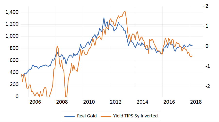
Source: BSIC, Data from Bloomberg
As it is possible to see from the graph, a relationship between 5 years TIPS and Gold exists. The following analysis has thus the objective to check whether or not it is possible to construct a trading strategy betting on the convergence of the two series which started to diverge in March 2016. Indeed, we want to verify whether the time series of Gold and Yield on 5years TIPS are cointegrated. Indeed, when two variables are cointegrated, their joint behavior can be predicted because their “randomness” is not independent but is instead generated by the same random process.
Then, If the result is positive, it would be possible to see at what “speed” these two series are expected to converge and if we can thus exploit their recent divergence to build a profitable trading strategy.
First, we need to check whether Gold and the yield on the 5 years TIPS (from now on 5YT) are non-stationary. We thus perform a Dickey-Fuller Test on Gold and 5yT and we cannot reject the null hypothesis that the two series are two random walks. In particular, we run the regression for both y=gold and y=5yT:![]()
Respectively the t-stat of the alphas are -1.48 and -0.67.
Given that the we cannot reject the null that the two series are random walks, the regression between the two series should lead to spurious results, unless the two series are cointegrated. Indeed, one way to test for cointegration is to check whether the residuals of the regression between the two series are stationary or not.
We thus performed the regression:![]()
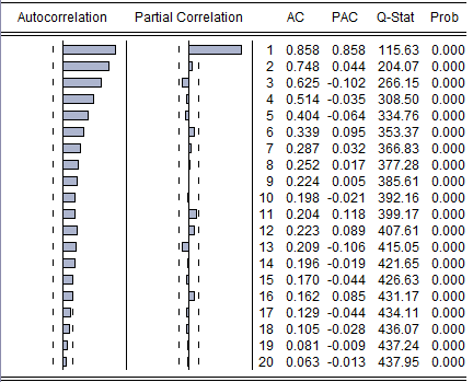
The plot of the estimated residuals and the ACF and PACF are:
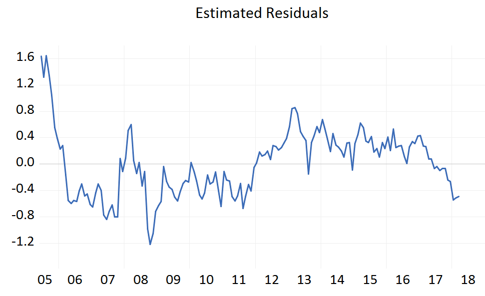
Source: BSIC, Data from bloomberg
The ACF, PACF and the graph seem to lead that the residuals are stationary and this was also confirmed by an additional DF test on the time series of the residuals. In particular, they look like they come from an AR(1) process with a really persistent lag coefficient. Indeed, the regression is not spurious, the two series are cointegrated and we can thus use a vector correction model (VECM) to predict the joint behavior of the series.
In order to choose the number of legs which gives the best tradeoff between reduction in the RSS of the model and risk of overfitting, we use information criteria on the unrestricted VAR(p) and then the optimal number of legs in the VECM will simply be p-1.
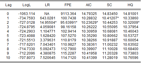
Source: BSIC, Data from Bloomberg
Given that the majority of the IC suggest that the number of p in the VAR is 2 we imply that the optimal p of the VEC is 1.
We thus estimate a VEC(1) on which we impose the restriction that the random walk process originates from the 5YT and then propagates to the Gold. The VEC is thus characterized. The final model is estimated to be:
∆(5YT) = 0*( – 2.57*5YT (-1) + 0.04*GOLD(-1) – 33.33 ) + 0.11*∆(5YT (-1)) – 0.0004*∆(GOLD(-1)) + 0.01 + εt
∆(GOLD) = – 1.26*( – 2.57*5YT (-1) + 0.04*GOLD(-1) – 33.36 ) + 46.17*∆(5YT (-1)) – 0.29*∆(GOLD(-1)) + 3.95 + εt
Where, as imposed, the error correction term is equal to zero in the ∆5YT series. The differentiated series ∆5YT is indeed always stationary while the ∆Gold series is stationary only if:
– 2.57*5YT (-1) + 0.04*GOLD(-1)= 33.36
When that is not the case, the negative alpha of the error correction term (-1.26) will adjust, on expectations, the levels of the two series, forcing Gold and 5YT to converge. We can thus use the VEC just estimated to forecast the series from April 2018 to December 2018 and see at which speed the two series are expected to converge. In particular, the forecast are the ones shown in the following graphs after the red line.
As expected from the parameters estimated, the two series are forecasted to converge but at a very slow pace. In particular, the forecasts suggest that the two series should increase but the inverted yield should increase (yield should decrease) at a faster pace than Gold. Regardless, the error correction term is small and thus, betting on the convergence of the series, may be very risky given that the volatility of the errors is very high with respect to the error correction term. Indeed, the spread between the two series may widen for many periods before converging. As a consequence, the trader may experience big losses, and thus margin calls, before it would be able to enjoy any profit.
To conclude, even if, on expectations, the two series are expected to converge, the risk that that they will widen too much before is very high and thus a hypothetical trading strategy on the convergence may be too risky to implement.


0 Comments